-
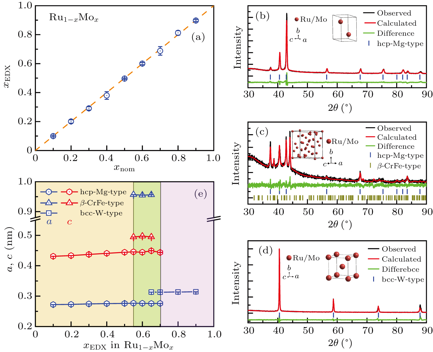
Figure 1. (a) Relationship between the nominal concentration of Mo xnom and the actual one xEDX determined by EDX in Ru1−xMox (x = 0.1–0.9) polycrystals. (b)–(d) Room-temperature PXRD patterns and refinements for Ru0.5Mo0.5, Ru0.4Mo0.6 and Ru0.1Mo0.9, respectively. (e) The lattice parameters a and c as a function of Mo content in Ru1−xMox.
-
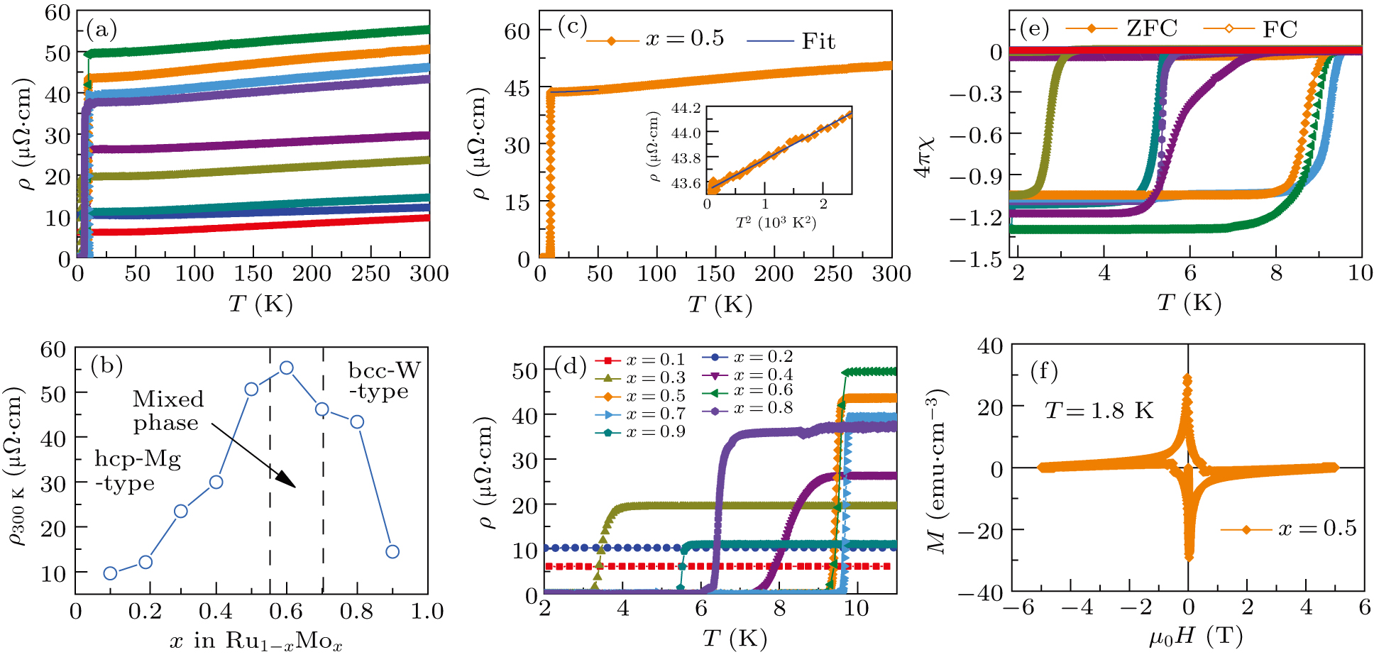
Figure 2. (a) Temperature dependence of electrical resistivity ρ(T) for Ru1−xMox (x = 0.1–0.9) polycrystals at zero field. (b) ρ300 K as a function of x. (c) The ρ(T) of Ru0.5Mo0.5 polycrystal at zero field. Inset: enlarged view of the fit in the range of 2–50 K. The blue solid lines represent the fits using the formula ρ(T) = ρ0 + AT2. (d) Enlarged view of ρ(T) below T = 11 K. (e) Temperature dependence of magnetic susceptibility 4πχ(T) measured at 1 mT with ZFC and FC modes. (f) The magnetization hysteresis loop measured at T = 1.8 K for the sample with x = 0.5. The color code in all figures except (b) is the same.
-
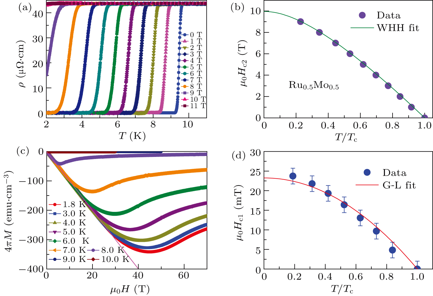
Figure 3. (a) The ρ(T) as a function of temperature at various fields for Ru0.5Mo0.5. (b) Temperature dependence of μ0Hc2(T). The green solid line represents the fit using the WHH formula. (c) Low-field dependence of magnetization 4πM(μ0H) at various temperatures below Tc. The pink solid line represents the Meissner line. (d) μ0Hc1(T) as a function of T/Tc. The red line represents the fit using the G-L equation.
-
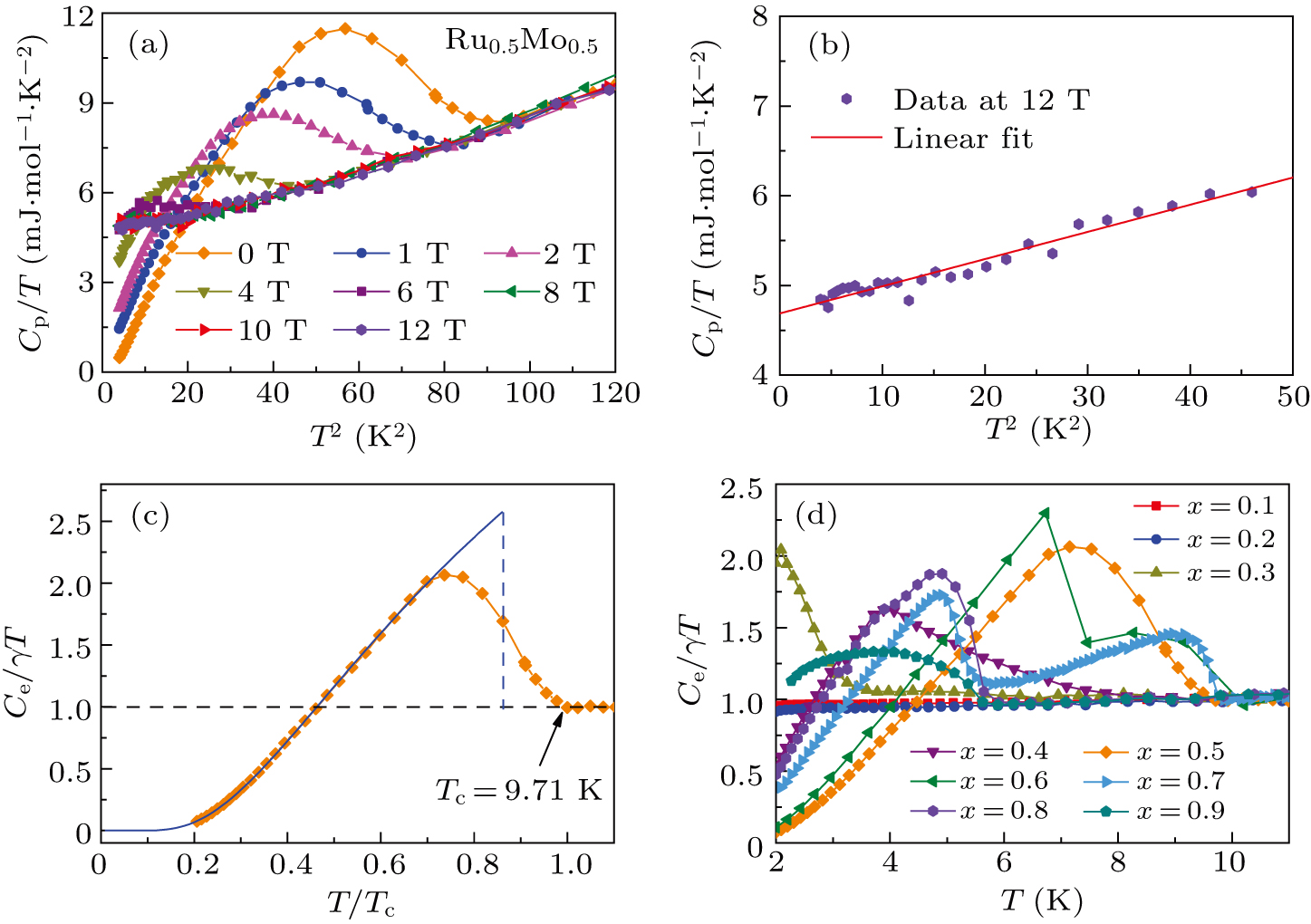
Figure 4. (a) The Cp/T vs. T2 at various fields for Ru0.5Mo0.5. (b) Cp/T vs. T2 at μ0H = 12 T. The red solid line represents the linear fit using the equation Cp(T)/T = γ + βT2. (c) Temperature dependence of electronic specific heat plotted as Ce/(γT) vs.
-
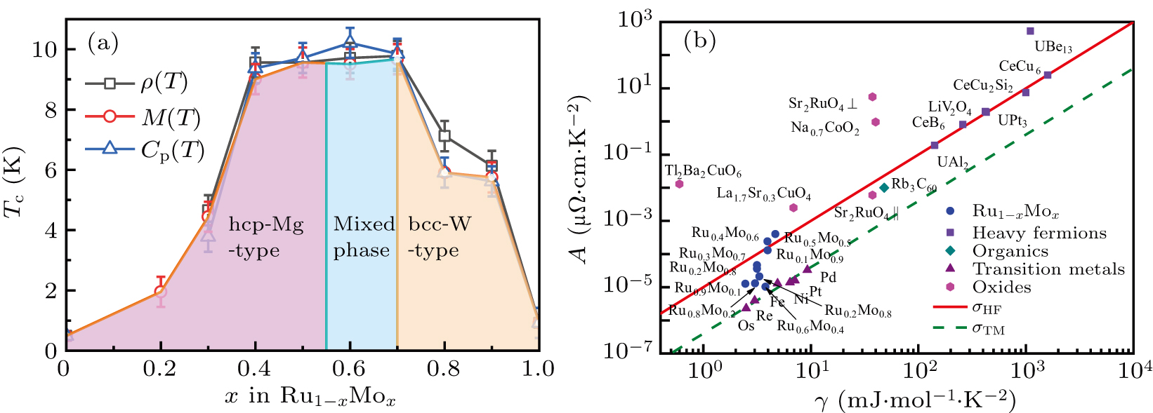
Figure 5. (a) Superconducting phase diagram of the Ru1−xMox. (b) Kadowaki–Woods plot for various superconductors. The red solid line represents σHF = 10 μΩ⋅cm⋅mol2⋅K2⋅J−2 and the green dashed line represents σTM = 0.4 μΩ⋅cm⋅mol2⋅K2⋅J−2.
Figure
5 ,Table
2 个