
 首页
首页 登录
登录 注册
注册


 下载:
下载:
-
人类社会的经济发展导致能源的消耗与日俱增, 其代价是不可再生能源的逐渐枯竭以及全球变暖凸显. 事实上, 工农业生产过程中产生的大量废热散失在空气中, 这造成了大量的能源浪费和环境污染. 因此, 将大量废热转变成有用的电能已经成为一个重要科学问题, 这也是热电效应(又称塞贝克效应(Seebeck effect))近年来引起了人们普遍关注的重要原因. 根据热电效应原理, 人们可以利用热电材料的温度梯度驱动材料内部的载流子从热端向冷端运动, 进而在材料的两端形成一个温差电动势, 这就实现了热电转换. 表征热电转换效率的物理量被称为热电品质因子
$ ZT $ , 其表达式为$ ZT = S^{2}G T/\kappa $ , 其中, S为塞贝克系数 (即热功率), G为电导, κ为热导, T是系统的平均温度. 值得注意的是, 传统的块体材料 的热电转换效率无法突破瓶颈1, 即$ ZT\leqslant 1 $ . 这构成了制约块体热电材料不能够大面积商业应用的一个关键因素.为了提高材料的热电品质因子
$ ZT $ , 人们在理论与实验方面付出了大量努力. 研究表明纳米材料不仅能够实现热电转换效率的显著增强, 而且对纳米结构热电效应的探究也有助于突破维德曼-弗兰兹定律的束缚[1,2]. 在过去的二十多年里, 人们在量子点[3-5]、量子线[6-8]、分子结[9,10]、石墨烯[11-14]、拓扑绝缘体[15,16]等纳米系统的热电效应方面开展了大量的研究工作, 一些新的物理现象被相继发现, 并且对其背后的物理机制也给出了深入阐释, 这些结果表明纳米结构在热电转换方面具有巨大的潜在应用价值. 在上述纳米体系中, 由金属-量子点-超导体构成的混合型量子点结构以其特有热电输运行为引起了人们广泛关注. 在传统观念里, 由于超导体电极的存在, 由金属-超导构成的混合系统必然伴随有安德列也夫反射(Andreev reflection) 现象的发生, 安德列也夫反射过程中伴随的电子-空穴对称性会极大地抑制热电效应. 然而, 如果借助于某种手段破坏输运过程中的电子-空穴对称性, 人们仍然能够得到非常显著的热电行为, 这为利用超导体特性实现热电转换指明了方向[17]. Hwang等[18]研究了铁磁-量子点-超导体混合型系统的热电输运, 他们发现铁磁电极的自旋极化和量子点上的塞曼劈裂能够导致非常大的热功率. 此外, 在金属(或铁磁)-量子点-超导体混合型结构中, 存在显著的热电二极管效应[19]. Trocha和Barnas[20]探究了一个铁磁-量子点-超导体的热电输运, 发现准粒子隧穿能够导致较大的热功率和热电品质因子. Michalek等[21]提出了一个基于超导体和量子点的三端混合型结构模型, 研究结果表明安德列也夫束缚态对于热功率存在间接影响, 但这种非直接影响具有潜在的应用价值. 此外, 借助于铁磁-量子点-超导体混合型结构的热功率, 人们可以实现超导体内电子奇数频率配对机制的热电探测[22,23].另一方面, 与单量子点结构相比, 双量子点结构因具有较多的自由度能够展现出更为丰富的物理特征. 在量子输运方面, 双量子点系统的电流具有Aharonov-Bohm振荡特征[24-26], 其电导谱也能够呈现出Fano干涉以及Kondo效应[27,28]. 在超导-双量子点-超导结构中, 不仅能够实现约瑟夫森流的
$ 0-\pi $ 转变, 而且约瑟夫森流也呈现出交换效应[29]. 双量子点具有操控自旋的自旋阀功能以及用于马约拉纳(Majorana) 费米子的探测[30,31]. 借助金属-量子点-超导体混合结构, 人们可以操控Andreev输运和库珀对的劈裂[32]. 而在混合型双量子点系统的热电效应方面, Yao等[33]研究了一个双量子点混合型系统的热电行为, 他们详细讨论了系统参数对热电量的影响, 并提出了利用外部磁通调控系统热电转换效率的方法. 利用一个含有超导电极的混合型双量子点Aharonov-Bohm干涉仪, 不仅能够实现维德曼-弗兰兹定律的强烈违背, 而且产生了显著的自旋相关的热电输运行为[34]. 在一个金属-双量子点-超导体的三端混合型结构中, 系统的非局域电子-空穴对称性的破坏会导致非局域热电效应的出现[35]. 此外, 含有超导体电极的量子点混合型结构可以用来设计热机或制冷机, 进而实现热-功转换的功能[36,37]. 由此可见, 金属-量子点-超导体混合型系统在热电转效率方面具有巨大的应用潜力.众所周知, 自旋-轨道耦合作用源于相对论效应. 固体材料中的自旋-轨道耦合作用包括Rashba自旋-轨道耦合与Dressalhaus自旋-轨道耦合两种类型, 前者源于结构反演不对称性, 后者是体反演不对称性导致的. 自旋-轨道耦合为操控量子材料中的电子自旋行为提供了物理基础. 考虑自旋-轨道相互作用, 研究发现金属-双量子点-超导体混合型结构(见图1)的热电效应鲜有研究, 而且自旋-轨道耦合效应如何影响上述混合结构的热电输运行为亟待揭示. 基于以上论述, 本文详细讨论了混合型量子点系统热电输运行为与系统参数的关系, 发现该混合系统不仅存在维德曼-弗兰兹定律的违背, 而且能够实现热电性能的显著增强. 通过调制参数, 系统能够产生纯自旋塞贝克效应, 这为产生纯自旋流器提供了一条有效途径. 此外, 本文也分析了这个混合型系统的热-功转换性质. 这些结果有助于深入理解混合型双量子点系统的热电输运及其热力学特征.
-
本文所考虑的含自旋-轨道耦合作用的混合型双量子点系统如图1 所示. N与S分别表示金属电极和超导电极, 量子点1和2分别与两个电极相接触. 整个系统的哈密顿量为
$ H = H_{{\mathrm{N}}}+H_{{\mathrm{S}}}+ H_{{\mathrm{C}}}+H_{{\mathrm{T}}} $ , 其中$ H_{{\mathrm{N}}} $ 表示金属电极的哈密顿量:式中,
$ a^{\dagger}_{{\mathrm{N}}k\sigma} $ ($ a_{{\mathrm{N}}k\sigma} $ ) 表示在金属电极内一个能量为$ \varepsilon_{k{\mathrm{N}}} $ 、动量为k和自旋为σ的电子的产生 (湮灭) 算符.$ H_{{\mathrm{S}}} $ 为超导电极的哈密顿量, 其具体形式表示为其中
$ a^{\dagger}_{{\mathrm{S}}k\sigma}(a_{{\mathrm{S}}k\sigma}) $ 是超导电极内电子的产生 (湮灭) 算符, 对应电子的能量为$ \varepsilon_{{\mathrm{S}}k} $ 、动量 (自旋) 为k ($ \sigma = \uparrow, \downarrow $ ).$ \varDelta > 0 $ 表示BCS超导体的能隙.$ H_{{\mathrm{C}}} $ 表示由两个量子点构成的中心区域的哈密顿量, 即方程(3) 中的
$ \varepsilon_{i\sigma} = \varepsilon_{i}+\sigma\varDelta_{z} $ 表示量子点的能级 (i = 1, 2), 其中$ \varepsilon_{i} $ 表示量子点的裸能级,$ \varDelta_{z} = \mu_{{\mathrm{B}}}B_{z} $ 为塞曼能,$ \mu_{{\mathrm{B}}} $ 为玻尔磁子.$ d^{\dagger}_{i\sigma}(d_{i\sigma}) $ 是量子点电子的产生 (湮灭) 算符, 其自旋为σ.$ t_{{\mathrm{c}}} $ 表示两个量子点之间的耦合强度. θ是有效的自旋-轨道耦合场$ |{\alpha}| = \alpha $ 与外磁场的夹角$ {{\boldsymbol{B}}} = (0, B_{z}) $ ,${\boldsymbol{ \sigma}}_{x} $ 和$ {\boldsymbol{\sigma}}_{z} $ 是自旋空间的泡利矩阵. 系统哈密顿量的最后一项$ H_{{\mathrm{T}}} $ 代表量子点与两个电极之间的隧穿耦合:其中,
$ V_{1 k} $ ($ V_{2 k} $ ) 表示量子点1(2)与电极N(S)的隧穿矩阵元. -
为了研究上述混合型双量子点系统的热电输运, 我们需要首先推导电流与热流公式. 从金属电极(N)流向超导电极(S)的自旋相关的电流可以表示为
式中,
$ N_{{\mathrm{e}}} = \varSigma_{k\sigma}a^{\dagger}_{{\mathrm{N}}k\sigma}a_{{\mathrm{N}}k\sigma} $ 是金属电极 (N) 的电子数算符. 借助非平衡格林函数和傅里叶变换公式, 自旋相关的电流$ I_{\sigma} $ 可以表示为式中,
$ \hat{\boldsymbol{\sigma}}_z $ 是一个扩展的$ 8\times8 $ 泡利第三矩阵. 方程(6)包含矩阵的求迹运算Tr$ \{\cdots\} $ .$ \{\cdots\} $ 内是一个$ 8\times8 $ 矩阵, 其中(11+55)表示这个矩阵对角元素的第1项与第5项相加, 进而能够给出自旋向上电流公式. 同理, (33+77)表示自旋向下电流的求迹运算.$ G^{r, a, < }(\varepsilon) $ 分别是南部表示$ \varPhi^{\dagger} = (d^{\dagger}_{1\uparrow},d_{1\downarrow}, d^{\dagger}_{1\downarrow}, d_{1\uparrow}, d^{\dagger}_{2\uparrow}, d_{2\downarrow}, d^{\dagger}_{2\downarrow}, d_{2\uparrow}) $ 下混合系统的推迟、超前和小格林函数. 利用戴森方程, 推迟格林函数$ G^{r}(\varepsilon) $ 可以表示为其中
$ g^{r}(\varepsilon) $ 是中心区域 (不含两个电极) 的格林函数, 其表达式为其中A, C和D是子矩阵, 其表达式分别为
方程(7)中的
$ \varSigma^{r}_{{\mathrm{N}}} $ 和$ \varSigma^{r}_{{\mathrm{S}}} $ 表示金属电极与超导电极的自能项, 自能项主要用来描述中心区域与两个电极之间的耦合, 其表达式分别为在方程(12)和(13)中,
$ \varGamma^{{\mathrm{N}}} = 2\pi\varSigma_{k\sigma}|V_{1 k}|^{2}\delta(\varepsilon\;- \varepsilon_{{\mathrm{N}}k}) $ ($ \varGamma^{{\mathrm{S}}} = 2\pi\varSigma_{k\sigma}|V_{2 k}|^{2}N_{{\mathrm{S}}} $ ) 是线宽函数$ \varGamma_{{\mathrm{N}}} $ ($ \varGamma_{{\mathrm{S}}} $ )的矩阵元,$ N_{{\mathrm{S}}} $ 是超导体处于正常态时的态密度. 在宽带近似条件下,$ \varGamma^{{\mathrm{N}}} $ 和$ \varGamma^{{\mathrm{S}}} $ 可看作常数. 0为$ 4\times4 $ 零矩阵.$ \rho(\varepsilon) $ 表示修正后的超导体态密度, 其具体形式为方程(6) 中的
$ F_{{\mathrm{N}}} $ 具体形式为推迟格林函数
$ G^{{\mathrm{r}}}(\varepsilon) $ 与超前格林函数$ G^{{\mathrm{a}}}(\varepsilon) $ 的关 系为$ [G^{{\mathrm{r}}}(\varepsilon)]^{\dagger} = G^{{\mathrm{a}}}(\varepsilon) $ , 于是小格林函数为$ G^{ < }(\varepsilon) = G^{{\mathrm{r}}}(\varepsilon)({\mathrm{i}}F_{{\mathrm{N}}}\varGamma_{{\mathrm{N}}} \;+\; {\mathrm{i}}f_{{\mathrm{S}}}\varGamma_{{\mathrm{S}}})G^{{\mathrm{a}}}(\varepsilon) $ . 其中,$ f(\varepsilon\mp\mu_{{\mathrm{N}}}) = [\exp((\varepsilon\mp\mu_{{\mathrm{N}}})/k_{{\mathrm{B}}}T_{{\mathrm{N}}}) + 1]^{-1} $ 以及$ f_{{\mathrm{S}}}(\varepsilon) = [\exp(\varepsilon/ k_{{\mathrm{B}}}T_{{\mathrm{S}}}) +1]^{-1} $ 分别为金属电极和超导电极的费米分布函数,$ k_{{\mathrm{B}}} $ 为玻尔兹曼常数,$ T_{{\mathrm{N}}} $ 和$ T_{{\mathrm{S}}} $ 分别为金属电极和超导电极的温度,$ \mu_{{\mathrm{N}}} $ 是金属电极的化学势, 而我们设超导电极的化学势$ \mu_{{\mathrm{S}}} = \mu = 0 $ .将方程(12)—(15)以及
$ G^{ < }(\varepsilon) $ 代入方程(6), 可得方程(16)和(17)中的
$ T_{A\sigma}(\varepsilon) $ 和$ T_{Q\sigma}(\varepsilon) $ 分别表示自旋相关的安德列也夫反射系数和准粒子透射系数, 其具体形式为其中
$ \tilde{\rho}(\varepsilon) = |\varepsilon|\theta(|\varepsilon|-\varDelta)/\sqrt{\varepsilon^{2}-\varDelta^{2}} $ ,$ G^{{\mathrm{r}}}_{ij}(\varepsilon) $ 是推迟格林函数$ G^{{\mathrm{r}}}(\varepsilon) $ 的矩阵元.对于从金属电极流出的热流而言, 可得
同样, 利用非平衡格林函数与傅里叶变换, 我们能够得到:
方程(23) 可以进一步化简为
-
令超导体的温度为
$ T_{{\mathrm{S}}} = T $ , 并且设金属电极的化学势和温度分别为$ \mu_{{\mathrm{N}}} = \mu_{{\mathrm{S}}}+\delta\mu = {\mathrm{e}}\delta V $ 和$ T_{{\mathrm{N}}} = T+\delta T $ , 其中$ \delta V $ 为小偏压. 在线性响应区域内, 将电流和热流写为如下形式[20]:式中,
$ L_{12\sigma}\neq L_{21\sigma} $ 源于磁场破坏了时间反演对称性.$ f(\varepsilon) = f(\varepsilon, \mu, T) $ 为平衡态下的费米分布函数.利用方程(28)的昂萨格系数, 可求得表征系统热电特征的热电系数 (也称热电量). 当回路中的电流
$ I_{\sigma} = 0 $ 时, 自旋相关的热功率$ S_{\sigma} $ 被定义为因此, 电荷热功率
$ S_{{\mathrm{c}}} $ 和自旋热功率$ S_{{\mathrm{s}}} $ 可以写为当
$ \delta T = 0 $ 时, 利用方程(26), 可得自旋相关的电导为这样, 电荷电导
$ G_{{\mathrm{c}}} $ 和自旋电导$ G_{{\mathrm{s}}} $ 表示为热导被定义为
进一步, 电荷热电品质因子
$ Z_{{\mathrm{c}}}T $ 和自旋电荷品质因子$ Z_{{\mathrm{s}}}T $ 被定义为式中,
$ \kappa_{{\mathrm{ph}}} $ 表示声子对热导的贡献, 由于系统处于低温区域,$ \kappa_{{\mathrm{ph}}} $ 的贡献可以忽略不计. 上述热电系数为进一步分析混合型系统的热电输运行为提供了有力工具. -
本节借助于上述热电系数公式进行数值计算, 并详细讨论金属-双量子点-超导体混合型系统的热电输运行为. 为了研究问题的方便起见, 选取超导电极的能隙Δ作为能量单位 (所有能量相关物理量均以Δ为单位), 并且设量子点与两个电极之间具有对称性耦合, 即
$ \varGamma^{{\mathrm{N}}} = \varGamma^{{\mathrm{S}}} = 0.1\varDelta $ . 通篇文章, 量子点之间的耦合强度被选取为$ t_{{\mathrm{c}}} = \varDelta $ .为了更好地理解含自旋-轨道耦合的混合型双量子点系统的热电输运特征, 设
$ \varepsilon_{1} = \varepsilon_{2} = \varepsilon_{{\mathrm{d}}} $ , 并且在图2给出了电荷热电系数随温度$ k_{{\mathrm{B}}}T $ 和能级$ \varepsilon_{{\mathrm{d}}} $ 的演化行为. 图2(a)呈现了电导$ G_{{\mathrm{c}}} $ 作为$ k_{{\mathrm{B}}}T $ 和$ \varepsilon_{{\mathrm{d}}} $ 函数的演化斑图, 电导$ G_{{\mathrm{c}}} $ 关于费米能级$ \varepsilon_{{\mathrm{d}}} = 0 $ 具有明显的对称性. 在低温条件下,$ G_{{\mathrm{c}}} $ 具有单峰(中心峰)结构, 这主要源于安德列也夫输运的贡献. 随着温度的升高, 中心峰明显降低, 更多的边峰出现在能隙之外, 这种行为能被更好地展示在对于不同温度的电导截面图中(见图2(a')). 在物理上, 上述行为主要源于温度的升高导致能隙之外的更多准粒子参与热电输运. 事实上, 热导$ \kappa_{{\mathrm{e}}} $ 仅仅取决于准粒子隧穿的贡献. 因此, 在低温时,$ \kappa_{{\mathrm{e}}} $ 几乎为零(见图2(b)). 随着温度的升高, 热导的线型呈现出复杂的结构, 不仅热导峰的强度增大, 而且在能隙之外呈现出更多的边峰(见图2(b')). 从图2(c)可以看出, 电荷塞贝克系数(电荷热功率)关于费米能级$ \varepsilon_{{\mathrm{d}}} = 0 $ 呈现出反对称结构,$ S_{{\mathrm{c}}} > 0 $ ($ S_{{\mathrm{c}}} < 0 $ )分别对应空穴(电子)型载流子的贡献. 不同温度截面图清楚地显示出存在多个电子-空穴对称点, 在对称点处$ S_{{\mathrm{c}}} = 0 $ (见图2(c')). 此外, 温度的升高会导致热功率$ S_{{\mathrm{c}}} $ 的峰(谷)逐渐远离能隙区($ |\varDelta| = 1 $ ), 这意味着更多能隙之外的准粒子由于温度升高被激发进而参与热电输运过程. 根据热电品质因子$ Z_{{\mathrm{c}}}T $ 表达式(34), 可以发现热功率的演化行为能够定性地折地折射到热电品质因子上(图2(d)). 由于$ Z_{{\mathrm{c}}}T $ 正比正比于$ k_{{\mathrm{B}}}T $ , 在通常情况下, 随着温度的升高会使$ Z_{{\mathrm{c}}}T $ 增强增强. 但这个混合型双量子点的$ Z_{{\mathrm{c}}}T $ 对对$ \kappa_{{\mathrm{e}}} $ 的响的响应大于$ k_{{\mathrm{B}}}T $ . 这样, 随着温度的升高,$ Z_{{\mathrm{c}}}T $ 呈现呈现出减小的趋势(图2(d')). 然而,$ Z_{{\mathrm{c}}}T $ 仍明仍明显大于1, 表明系统存在着强烈的维德曼-弗兰兹违背现象, 这意味着这个混合型系统能够实现较大的热电转换.下文主要聚焦于系统的自旋塞贝克输运行为. 图3(a)给出了自旋热功率
$ S_{{\mathrm{s}}} $ 在温度$ k_{{\mathrm{B}}}T $ 和能级$ \varepsilon_{{\mathrm{d}}} $ 构成的参数空间中的演化特征, 可以看出$ S_{{\mathrm{s}}} $ 具有明显的对称性结构, 温度的增加导致$ S_{{\mathrm{s}}} $ 的峰逐渐远离能隙. 随着能级$ \varepsilon_{{\mathrm{d}}} $ 的变化,$ \pm S_{{\mathrm{s}}} $ 交替出现, 这表明可以通过门电压调控自旋热功率$ S_{{\mathrm{s}}} $ , 进而控制热驱动自旋流的方向(图3(a')). 值得注意的是, 在一定的温度范围内可以实现升高温度进而增强自旋热电转换效率($ Z_{{\mathrm{s}}}T $ )的目的(图3(b)), 而且$ Z_{{\mathrm{s}}}T $ 也能够大于1 (图3(b')), 这些性质有助于设计基于自旋的热电器件.与磁场相关的塞曼能
$ \varDelta_{z} $ 作为一个重要的物理量能够显著影响系统的热电输运特征. 因此, 图4展示了热功率(热电转换效率)随着$ \varDelta_{z} $ 和$ \varepsilon_{{\mathrm{d}}} $ 的演化行为. 关于费米能级, 电荷热功率$ S_{{\mathrm{c}}} $ 与自旋热功率$ S_{{\mathrm{s}}} $ 分别呈现出反对称与对称的几何特征, 增强$ \varDelta_{z} $ 使得热功率($ S_{{\mathrm{c}}} $ 和$ S_{{\mathrm{s}}} $ )在费米能级附近的变化更为剧烈(图4(a)—(c)). 重要的是, 调制$ \varepsilon_{{\mathrm{d}}} $ 可以使$ S_{{\mathrm{c}}} = 0 $ (实线)但$ S_{{\mathrm{s}}}\neq 0 $ (虚线), 如图4(c)中的箭头所示, 这样能够得到一种纯自旋塞贝克效应, 可以利用这个效应制造一种纯自旋流发生器. 热电转换效率$ Z_{{\mathrm{c}}}T $ 和$ Z_{{\mathrm{s}}}T $ 的演化斑图均相对于费米能级呈现出明显的对称结构(图4(d), (e)), 而且增强$ \varDelta_{z} $ 更易于提高热电转换效率$ Z_{{\mathrm{c}}}T $ , 如图4(f)中的实线. 有趣的是, 增大$ \varDelta_{z} $ 可以实现巨大的自旋热电转换效率$ Z_{{\mathrm{s}}}T $ , 如图4(f)中的红色虚线, 意味着这个混合双量子点系统可作为实现较大自旋热电转换器件的候选者.事实上, 热电载流子的自旋输运行对于自旋-轨道耦合作用非常敏感. 因此, 图5呈现了自旋热电系数(
$ S_{{\mathrm{s}}} $ 和$ Z_{{\mathrm{s}}}T $ )对于自旋-轨道耦合强度α与能级$ \varepsilon_{{\mathrm{d}}} $ 的依赖性关系. 在参数空间(α,$ \varepsilon_{{\mathrm{d}}} $ )内,$ S_{{\mathrm{s}}} $ 和$ Z_{{\mathrm{s}}}T $ 依然相对于费米能级具有明显的对称性特征. 而且随着能级$ \varepsilon_{{\mathrm{d}}} $ 的变化,$ S_{{\mathrm{s}}} $ 展现出明显的振荡特征(见图5(a')).$ S_{{\mathrm{s}}} $ 的行为能够定性地反映到$ Z_{{\mathrm{s}}}T $ 演化行为上(见图5(b')). 在混合型双量子点系统中, 塞曼场会使量子点的能级产生劈裂, 这会导致超导能隙之外的准粒子出现自旋极化的热电输运行为. 但随着自旋-轨道耦合作用的出现, 自旋热电系数会逐渐减弱. 这源于自旋-轨道耦合作用与塞曼场的竞争机制, 因此α的增强会逐渐抑制载流子的自旋热电输运行为. 通过调制量子点能级与自旋-轨道耦合强度, 图5能够为获得满足实际需要的自旋热电系数提供一定的物理信息.为了能够深入理解量子点能级(
$ \varepsilon_{1} $ 与$ \varepsilon_{2} $ )如何调控热电输运行为, 图6给出了量子点能级空间下热功率与热电品质因子的演化图. 与图2—图5相比较, 在图6(a)和图6(b)中, 电荷热功率$ S_{{\mathrm{c}}} $ 和自旋热功率$ S_{{\mathrm{s}}} $ 随着$ \varepsilon_{1} $ 与$ \varepsilon_{2} $ 演化并未呈现出明显的对称性分布. 但$ S_{{\mathrm{c}}} $ 和$ S_{{\mathrm{s}}} $ 的清晰演化斑图为获得满足实际应用需要的热功率($ S_{{\mathrm{c}}} $ 与$ S_{{\mathrm{s}}} $ )提供了物理上允许的参数空间. 从图6(c), (d)可以看出, 热功率的这种非对称性分布也部分地反映在了热电品质因子($ Z_{{\mathrm{c}}}T $ 和$ Z_{{\mathrm{s}}}T $ )的分布上. 调制两个量子点的能级, 我们可以找到实现违背维德曼-弗兰兹定律的区域, 进而实现热电性能的增强(图6(c)). 进一步研究表明量子点能级的调控提供了实现大自旋热电转换效率$ Z_{{\mathrm{s}}}T $ 的可能性(图6(d)).最后, 我们分析了这个混合型双量子点结构的热-功转换性质. 令热力学力
$ X_{1} = {{e}}\delta V/k_{{\mathrm{B}}}T $ 和$ X_{2} = \delta T/k_{{\mathrm{B}}}T^{2} $ , 方程(26)和(27)可以表示为其中,
$ {\cal{L}}_{11} = \mathrm{\mathit{e}}k_{\mathrm{B}}TL_{11} $ ,$ {\cal{L}}_{12} = {{e}}k_{{\mathrm{B}}}T L_{12} $ ,$ {\cal{L}}_{21} = k_{{\mathrm{B}}}T L_{21} $ 和$ {\cal{L}}_{22} = k_{{\mathrm{B}}}T L_{22} $ . 将这个混合型量子点系统可以视为一个工作在线性响应区域的热机, 利用昂萨格方程(35), 热机的功率可以表示为$ P = ITX_{1} $ . 令$ \partial P/\partial X_{1} = 0 $ , 可得$ X^{\star}_{1} = -{\cal{L}}_{12} X_{2}/(2{\cal{L}}_{11}) $ , 将$ X^{\star}_{1} $ 代入功率P的表达式, 可得混合热机的最大功率[38]其中
$ \eta_{{\mathrm{c}}} = \delta T/T $ 为卡诺效率. 于是, 混合型热机在最大功率时的效率为[38]以
$ P_{0} = (k_{{\mathrm{B}}}\delta T)^{2}/h $ 和$ \eta_{{\mathrm{c}}} $ 为单位, 图7给出了 混合型热机的功率$ P_{{\mathrm{max}}} $ 与效率$ \eta_{{\mathrm{max}}P} $ 在能量空间 ($ \varepsilon_{1}, \varepsilon_{2} $ )的演化图形. 从图7(a)可以看出, 最大功率$ P_{{\mathrm{max}}} $ 的较大值主要集中在直线$ \varepsilon_{2} = \varepsilon_{1} $ 附近, 且在对角直线的两侧呈现出类对称分布特征, 当$ \varepsilon_{1} $ 和$ \varepsilon_{2} $ 的取值偏离直线$ \varepsilon_{2} = \varepsilon_{1} $ 时,$ P_{{\mathrm{max}}} $ 逐渐减小甚至消失. 令$ \delta = \varepsilon_{2}-\varepsilon_{1} $ 表示能级的失谐度, 当δ较小时,$ \varepsilon_{2} $ 与$ \varepsilon_{1} $ 越接近同步变化, 功率$ P_{{\mathrm{max}}} $ 更容易获得最大值. 因为$ \varepsilon_{2} $ 与$ \varepsilon_{1} $ 同步变化时, 电子倾向于能够实现协同输运. 相较而言, 效率$ \eta_{{\mathrm{max}}P} $ 演化行为较为复杂, 但其相对于直线$ \varepsilon_{2} = \varepsilon_{1} $ 也呈现出类对称分布, 而且在$ \varepsilon_{2} = \varepsilon_{1} $ 的两侧分布范围较大, 如图7(b)所示. 由于:所以
$ \eta_{{\mathrm{max}}P} $ 的演化可以定性地反映在$ Z_{{\mathrm{c}}}T $ 的变化上(见图6(c)). 众所周知, 对于一个热机而言, 其功率与效率不可能同时达到最优值, 这一固有特性也能够反映在混合型热机的热力学行为上面. 从效率分布可以看出,$ \eta_{{\mathrm{max}}P} $ 与$ P_{{\mathrm{max}}} $ 未呈现出同步演化行为, 即在$ P_{{\mathrm{max}}} $ 非常弱的某些区域,$ \eta_{{\mathrm{max}}P} $ 仍然具有较大值. 但是, 研究者们仍然可以通过调制量子点的能级 在一定程度上实现功率与效率的增强, 进而满足实际应用的需要. 当然, 本文仅仅给出了功率与效率在能量空间($ \varepsilon_{2}, \varepsilon_{1} $ )演化行为. 事实上, 人们可以分析功率与效率在($ k_{{\mathrm{B}}}T, \varepsilon_{{\mathrm{d}}} $ )、($ \varDelta_{z}, \varepsilon_{{\mathrm{d}}} $ )和($ \alpha, \varepsilon_{{\mathrm{d}}} $ ) 空间的演化特征, 进而得到其他的功能区间, 这构成了我们下一步的研究工作. -
基于非平衡格林函数方法和线性响应理论, 本文研究了一个含自旋-轨道耦合作用的金属-双量子点-超导体混合型系统的热电转换行为. 我们给出了昂萨格系数和热电系数表达式, 并详细阐述了这个混合型双量子点器件的热电输运与系统参数之间的关系. 电荷与自旋热电系数在参数(
$ \varepsilon_{{\mathrm{d}}} $ ,$ k_{{\mathrm{B}}}T $ )空间内具有明显的对称性特征, 温度的升高会致使Andreev输运的减小, 因此在能隙之内的电导峰降低, 但能隙之外边电导峰逐渐增强. 随着温度的升高, 能隙之外的更多准粒子参与热电输运, 这不仅会导致热导增强, 而且在远离能隙区产生较大的电荷热功率. 虽然热导的增大会导致热电效率($ Z_{{\mathrm{c}}}T $ )一定程度的减弱, 但$ Z_{{\mathrm{c}}}T $ 仍然大于1, 这意味着存在维德曼-弗兰兹定律的强烈违背. 随着温度的升高, 由于更多准粒子参与热电输运, 因此在远离能隙的区域,$ S_{{\mathrm{s}}} $ 具有较大值. 而且, 人们可以得到较大的自旋热电效率($ Z_{{\mathrm{s}}}T $ ). 热功率($ S_{{\mathrm{c}}} $ 和$ S_{s} $ )与热电品质因子($ Z_{{\mathrm{c}}}T $ 和$ Z_{{\mathrm{s}}}T $ ) 作为能级$ \varepsilon_{{\mathrm{d}}} $ 与塞曼能$ \varDelta_{z} $ 函数展现出了丰富的演化特征. 更为重要的是, 伴随着$ S_{{\mathrm{c}}} $ 的消失, 一个纯自旋塞贝克效应能够被产生, 这可以被用来设计纯自旋流热电发生器. 由于自旋-轨道耦合作用与塞曼场存在竞争机制, 这导致α的增大会逐渐削弱自旋热电系数的强度, 但对自旋-轨道耦合作用的调控能够为获得满足实际需要的自旋热电量提供有效途径. 热电系数在能量空间($ \varepsilon_{1} $ ,$ \varepsilon_{2} $ )演化图表明人们可以通过调制双量子点的能级实现热电转换效率的增强. 此外, 本文分析了混合型双量子点系统的热-功转换性质. 作为一个热机, 其功率与效率没有实现同步演化. 但在一些参数区域, 人们仍然可以获得满足实际需要的热力学性能.
含自旋-轨道耦合作用的金属-双量子点-超导体混合型系统的热电输运研究
Thermoelectric transport of normal metal-double quantum dots-superconductor hybrid system with spin-orbit coupling
-
摘要: 混合型量子点系统是研究热电转换机制的良好平台. 本文提出了一个含自旋-轨道作用的双量子点耦合金属和超导体构成的混合型系统模型, 并对其电荷以及自旋热电输运特征进行研究. 深入讨论了热电系数与系统参数之间的关系, 结果发现系统存在显著的维德曼-弗兰兹定律违背现象, 这有助于增强热电转换效率. 更重要的是, 由于存在超导体能隙外的准粒子隧穿, 这个混合型热电器件能够产生纯自旋塞贝克效应. 在实践上, 该效应可以被利用设计和制造一个纯自旋流发生器. 在线性响应机制下, 本文也讨论了该混合型热电系统作为一个热机的热力学性能. 本研究结果对于理解混合型热电系统的热电转换特征及其热力学性能具有理论和实践意义.Abstract: The normal metal-quantum dots-superconductor hybrid system is a good platform for studying the mechanism of thermoelectric conversion. In terms of non-equilibrium Keldysh Green’s function formalism and linear response theory, the charge and spin thermoelectric transport characteristics of a normal-double quantum dot-superconductor hybrid system with spin-orbit coupling are studied in this work. We delve into the relationship between thermoelectric coefficients and the system parameters, and find both charge and spin thermoelectric coefficients exhibit distinct symmetry in the parameter space composed of temperature and energy. The increase in temperature leads to a decrease in conductance within the energy gap, which is attributed to the reduction in Andreev transport. However, outside the energy gap, the conductance gradually increases, and the thermal conductance is gradually enhanced. This is because more quasiparticles outside the energy gap participate in thermoelectric transport, and a large charge thermopower is generated in the region far from the energy gap. It is found that the thermoelectric figure of merit is greater than 1, indicating a strong violation of the Wiedemann-Franz law. With the increase of temperature, the large spin thermopower as well as spin thermoelectric figure of merit can be obtained outside the energy gap. The charge (spin) thermopower and the thermoelectric figure of merit show the rich evolutionary characteristics as functions of energy level and Zeeman energy. With the disappearance of the charge thermopower, the spin thermopower still has a finite value, which leads to the emergence of a pure spin Seebeck effect. This is helpful for designing a pure spin current thermoelectric generator. Due to a competitive mechanism between the spin-orbit coupling effect and the Zeeman field, thermoelectric coefficients decrease with the strength of spin-orbit interaction increasing, but one still can obtain the spin thermoelectric quantities which meet the practical needs by regulating the strength of spin-orbit coupling and the Zeeman energy. The evolution pattern of the thermoelectric coefficientss in the energy space indicates that the enhancement of thermoelectric conversion efficiency can be achieved by modulating the energy levels of double quantum dots. In addition, this hybrid system can act as a heat engine to achieve the conversion of heat into work. Although its power and efficiency do not evolve synchronously, thermodynamic performance that meets practical needs can still be obtained in certain parameter regions. The research results of this work hold theoretical and practical significance for understanding the thermoelectric transport and thermodynamic performance of hybrid thermoelectric systems.
-
Key words:
- hybrid quantum dot system /
- spin-orbit coupling /
- thermoelectric transport /
- power and efficiency .
-

-
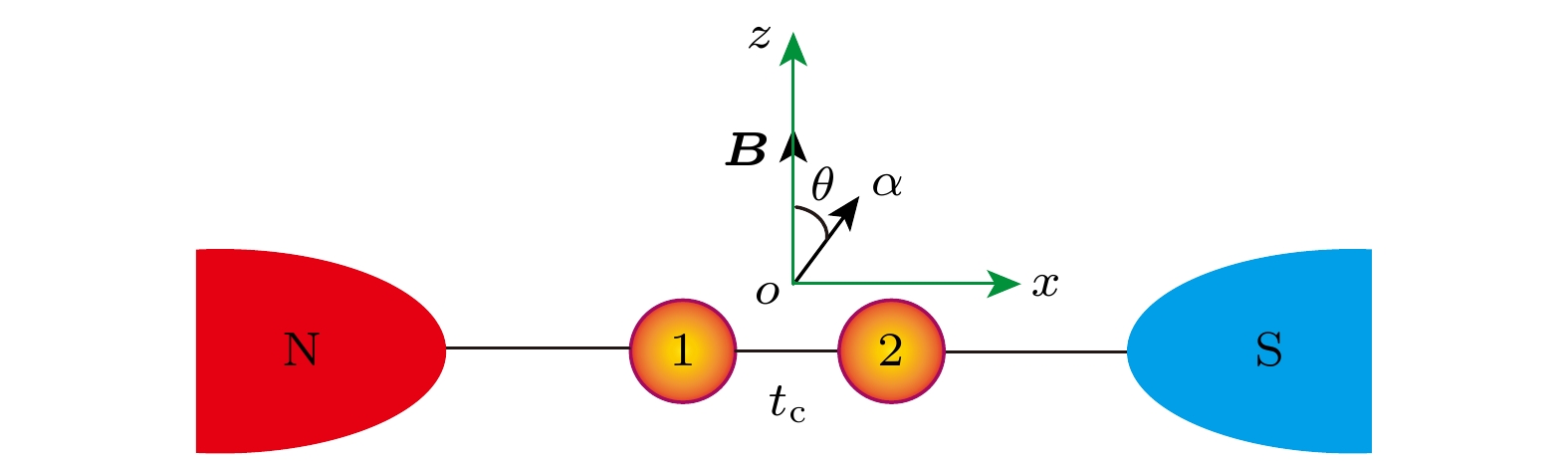
图 1 混合型双量子点结构模型, N表示与量子点1连接的金属电极, S表示与量子点2连接的超导电极,
$t_{{\mathrm{c}}}$ 为量子点之间的耦合强度, θ为自旋-轨道耦合场${\alpha}$ 与z轴方向的外磁场B 之间的夹角Figure 1. Model of hybrid double quantum dots, where N is a normal-metal electrode that is attached to the quantum dot 1, and S represents the superconducting electrode that is connected with the quantum dot 2,
$t_{{\mathrm{c}}}$ is the interdot coupling strength, and θ denotes the included angle between the spin-orbit coupling field${\alpha}$ and the external field B along the z axis.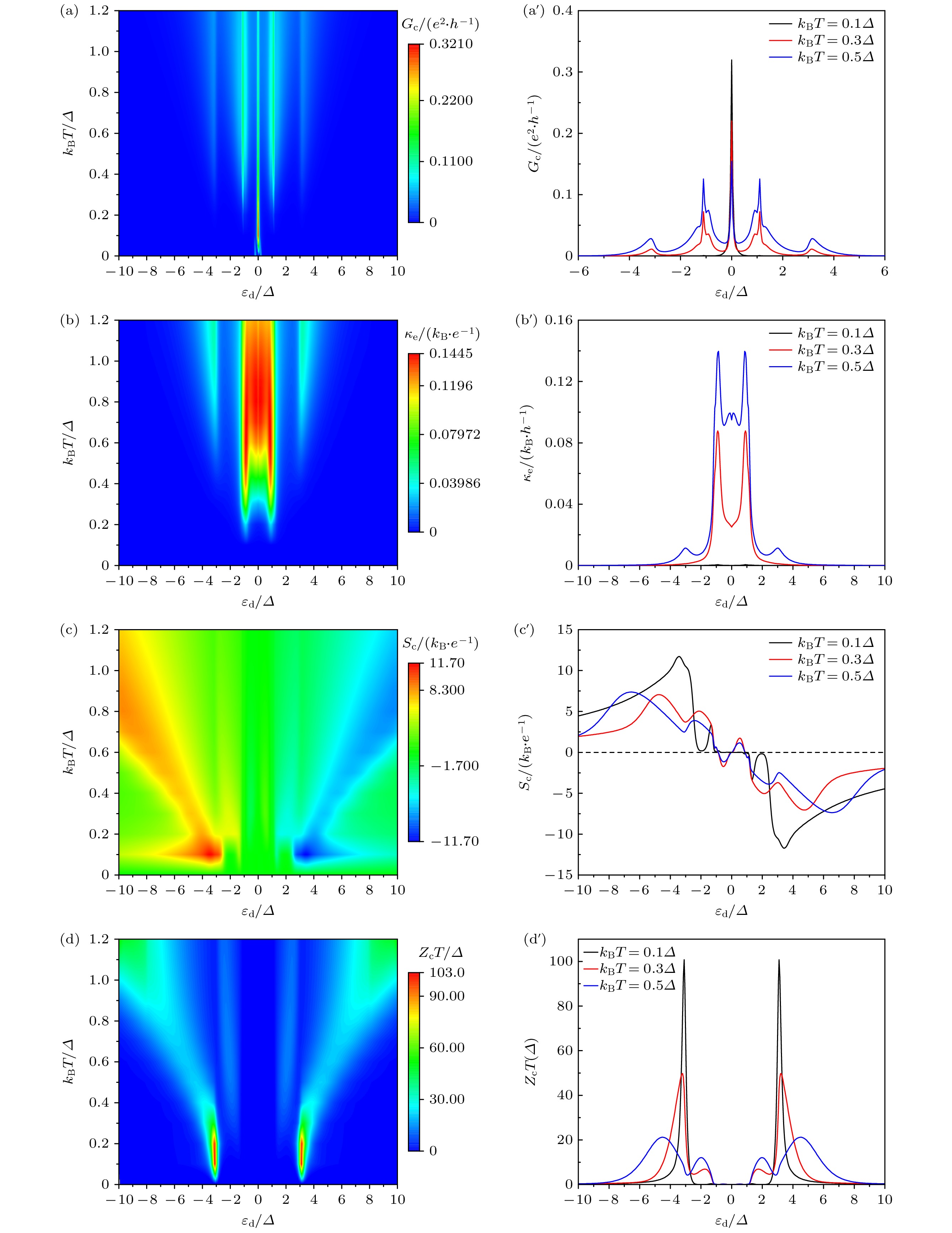
图 2 (a)电导
$G_{{\mathrm{c}}}$ 、(b)热导$\kappa_{{\mathrm{e}}}$ 、(c)热功率$S_{{\mathrm{c}}}$ 和 (d)品质因子$Z_{{\mathrm{c}}}T$ 作为能级$\varepsilon_{{\mathrm{d}}}$ 与温度$k_{{\mathrm{B}}}T$ 的函数; 不同温度条件下, (a')电导$G_{{\mathrm{c}}}$ 、(b')热导$\kappa_{{\mathrm{e}}}$ 、(c')热功率$S_{c}$ 和 (d')品质因子$Z_{{\mathrm{{\mathrm{c}}}}}T$ 的截面图; 其他参数$\alpha=0.2\varDelta$ ,$\varDelta_{z}=\varDelta$ 以及$\theta=\pi/2$ Figure 2. (a) Conductance
$G_{{\mathrm{c}}}$ , (b) heat conductance$\kappa_{{\mathrm{e}}}$ , (c) thermopower$S_{{\mathrm{c}}}$ and (d) figure of merit$Z_{{\mathrm{c}}}T$ as a function of the energy level$\varepsilon_{d}$ and temperature$k_{{\mathrm{B}}}T$ (left column); for different temperatures, the cross sections of (a') conductance$G_{{\mathrm{c}}}$ , (b') heat conductance$\kappa_{{\mathrm{e}}}$ , (c') thermopower$S_{{\mathrm{c}}}$ and (d') figure of merit$Z_{{\mathrm{c}}}T$ are shown; the other parameters are$\alpha=0.2\varDelta$ ,$\varDelta_{z}=\varDelta$ , and$\theta=\pi/2$ .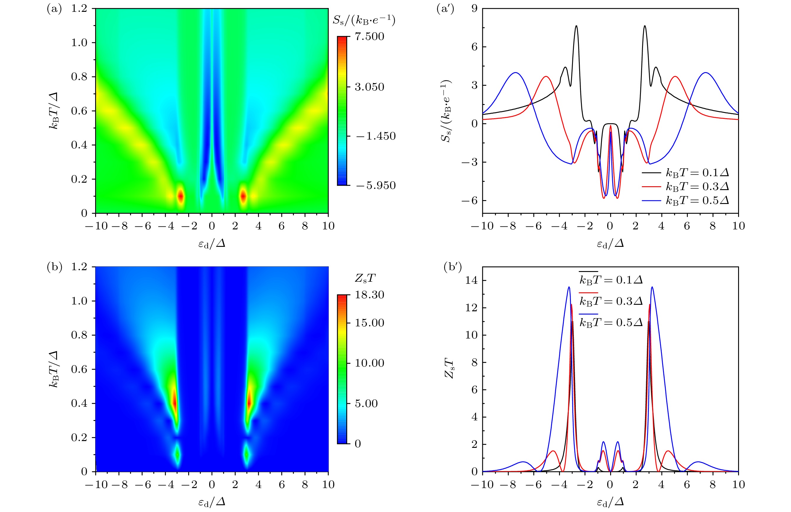
图 3 自旋热电系数(a)热功率
$S_{{\mathrm{s}}}$ 和 (b)品质因子$Z_{{\mathrm{s}}}T$ 作为能级$\varepsilon_{{\mathrm{d}}}$ 与温度$k_{{\mathrm{B}}}T$ 的函数. 不同温度条件下, (a')热功率$S_{{\mathrm{s}}}$ 和 (b') 品质因子$Z_{{\mathrm{s}}}T$ 的截面图; 其他参数$\alpha=0.2\varDelta$ ,$\varDelta_{z}=\varDelta$ 以及$\theta=\pi/2$ Figure 3. Spin thermoelectric coefficients (a) thermopower
$S_{{\mathrm{s}}}$ and (b) figure of merit$Z_{{\mathrm{s}}}T$ as a function of the energy level$\varepsilon_{{\mathrm{d}}}$ and temperature$k_{{\mathrm{B}}}T$ (left column). For different temperatures, the cross sections of (a') thermopower$S_{{\mathrm{c}}}$ and (b') figure of merit$Z_{{\mathrm{s}}}T$ are shown in the right column; the other parameters are$\alpha=0.2\varDelta$ ,$\varDelta_{z}=1\varDelta$ , and$\theta=\pi/2$ .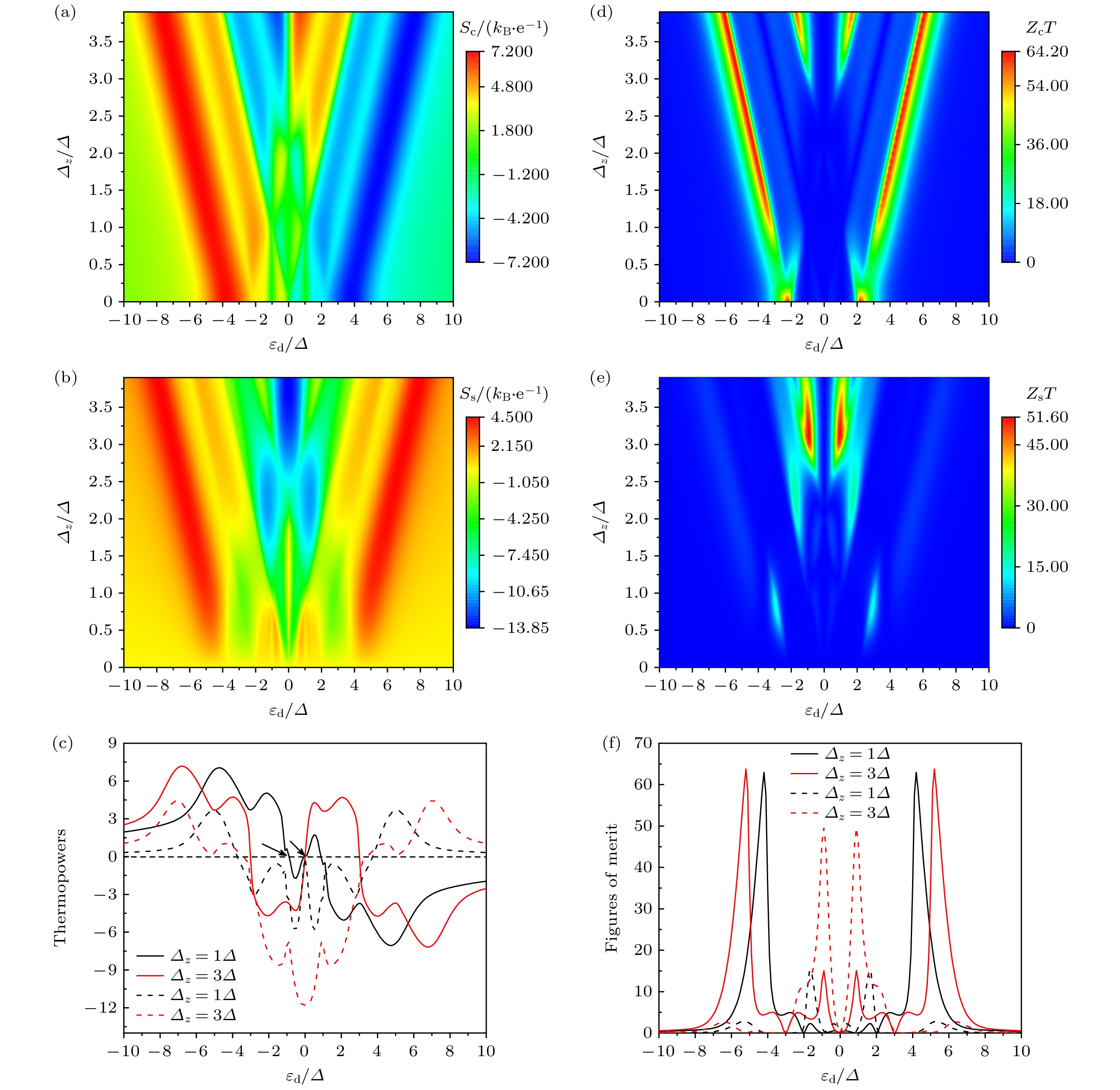
图 4 (a)电荷热功率
$S_{{\mathrm{c}}}$ 和(b)自旋热功率$S_{{\mathrm{s}}}$ 作为能级$\varepsilon_{{\mathrm{d}}}$ 与塞曼能$\varDelta_{z}$ 的函数; (c)不同塞曼能条件下,$S_{{\mathrm{c}}}$ (实线)和$S_{{\mathrm{s}}}$ (虚线)作为$\varepsilon_{{\mathrm{d}}}$ 的函数; (d)电荷品质因子$Z_{{\mathrm{c}}}T$ 和(e)自旋品质因子$Z_{{\mathrm{s}}}T$ 作为能级$\varepsilon_{{\mathrm{d}}}$ 与塞曼能$\varDelta_{z}$ 的函数; (f)不同塞曼能条件下,$Z_{{\mathrm{c}}}T$ (实线)和$Z_{{\mathrm{s}}}T$ (虚线)作为$\varepsilon_{{\mathrm{d}}}$ 的函数; 其他参数$\alpha=0.2\varDelta$ ,$k_{{\mathrm{B}}}T=0.3\varDelta$ 以及$\theta=\pi/2$ Figure 4. (a) Charge thermopower
$S_{{\mathrm{c}}}$ and (b) spin thermopower$S_{{\mathrm{s}}}$ as a function of the energy level$\varepsilon_{{\mathrm{d}}}$ and the Zeeman energy$\varDelta_{z}$ ; (c) for different Zeeman energies,$S_{{\mathrm{c}}}$ and$S_{{\mathrm{s}}}$ as a function of the energy level$\varepsilon_{{\mathrm{d}}}$ ; (d) charge figure of merit$Z_{{\mathrm{c}}}T$ and (e) spin figure of merit$Z_{{\mathrm{s}}}T$ as a function of the energy level$\varepsilon_{{\mathrm{d}}}$ and the Zeeman energy$\varDelta_{z}$ ; (f) for different Zeeman energies,$Z_{{\mathrm{c}}}T$ and$Z_{{\mathrm{s}}}T$ ) as a function of the energy level$\varepsilon_{{\mathrm{d}}}$ ; the other parameters are$\alpha=0.2\varDelta$ ,$k_{{\mathrm{B}}}T=0.3\varDelta$ , and$\theta=\pi/2$ .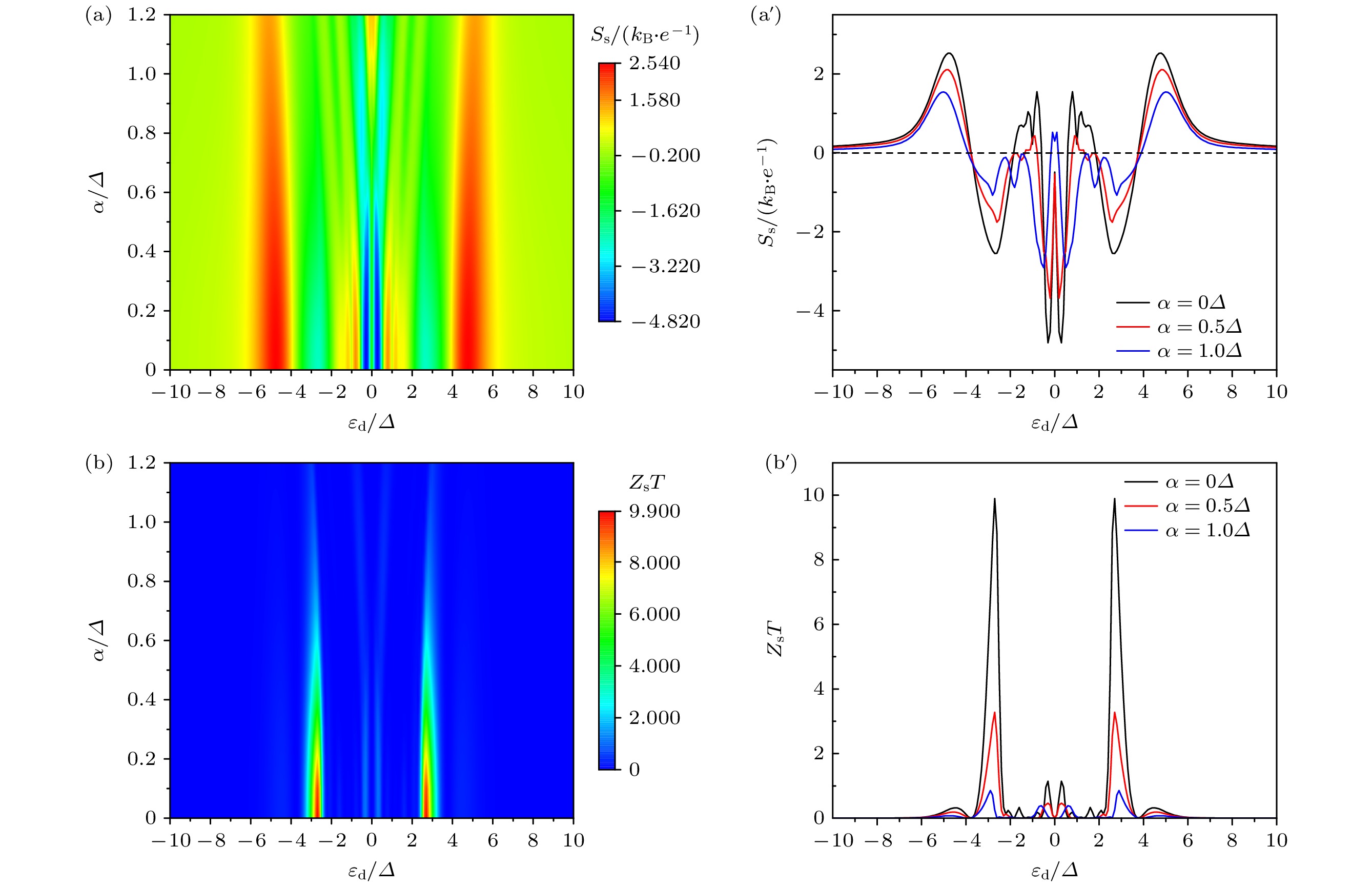
图 5 自旋热电系数(a)热功率
$S_{{\mathrm{s}}}$ 和 (b)品质因子$Z_{{\mathrm{s}}}T$ 作为能级$\varepsilon_{{\mathrm{d}}}$ 与自旋-轨道耦合强度α的函数; 不同α条件下, (a')热功率$S_{{\mathrm{s}}}$ 和 (b') 品质因子$Z_{{\mathrm{s}}}T$ 的截面图; 其他参数$\varDelta_{z}=0.5\varDelta$ ,$k_{{\mathrm{B}}}T=0.3\varDelta$ 以及$\theta=\pi/2$ Figure 5. Spin thermoelectric coefficients (a) thermopower
$S_{{\mathrm{s}}}$ and (b) figure of merit$Z_{{\mathrm{s}}}T$ as a function of the energy level$\varepsilon_{{\mathrm{d}}}$ and spin-orbit coupling strength α (left column); for different temperatures, the cross sections of (a') thermopower$S_{{\mathrm{c}}}$ and (b') figure of merit$Z_{{\mathrm{s}}}T$ are shown, the other parameters are$\varDelta_{z}=0.5\varDelta$ ,$k_{{\mathrm{B}}}T=0.3\varDelta$ , and$\theta=\pi/2$ .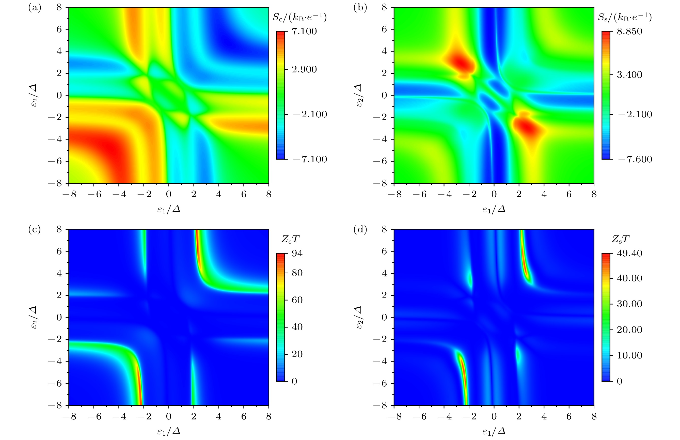
图 6 电荷热电系数(a)热功率
$S_{{\mathrm{c}}}$ 和 (b)品质因子$Z_{{\mathrm{c}}}T$ 作为量子点能级$\varepsilon_{1}$ 与$\varepsilon_{2}$ 的函数; 自旋热电系数 (c)热功率$S_{{\mathrm{s}}}$ 和 (d) 品质因子$Z_{{\mathrm{s}}}T$ 作为量子点能级$\varepsilon_{1}$ 与$\varepsilon_{2}$ 的函数; 其他参数为$\alpha=0.2\varDelta$ ,$\varDelta_{z}=\varDelta$ ,$k_{{\mathrm{B}}}T=0.3\varDelta$ 以及$\theta=\pi/2$ Figure 6. Charge thermoelectric coefficients (a) thermopower
$S_{{\mathrm{c}}}$ and (c) figure of merit$Z_{{\mathrm{c}}}T$ as a function of the quantum dot’s levels$\varepsilon_{1}$ and$\varepsilon_{2}$ ; spin thermoelectric coefficients (b) thermopower$S_{{\mathrm{s}}}$ and (d) figure of merit$Z_{{\mathrm{s}}}T$ as a function of the quantum dot’s levels$\varepsilon_{1}$ and$\varepsilon_{2}$ ; the other parameters are$\alpha=0.2\varDelta$ ,$k_{{\mathrm{B}}}T=0.3\varDelta$ , and$\theta=\pi/2$ .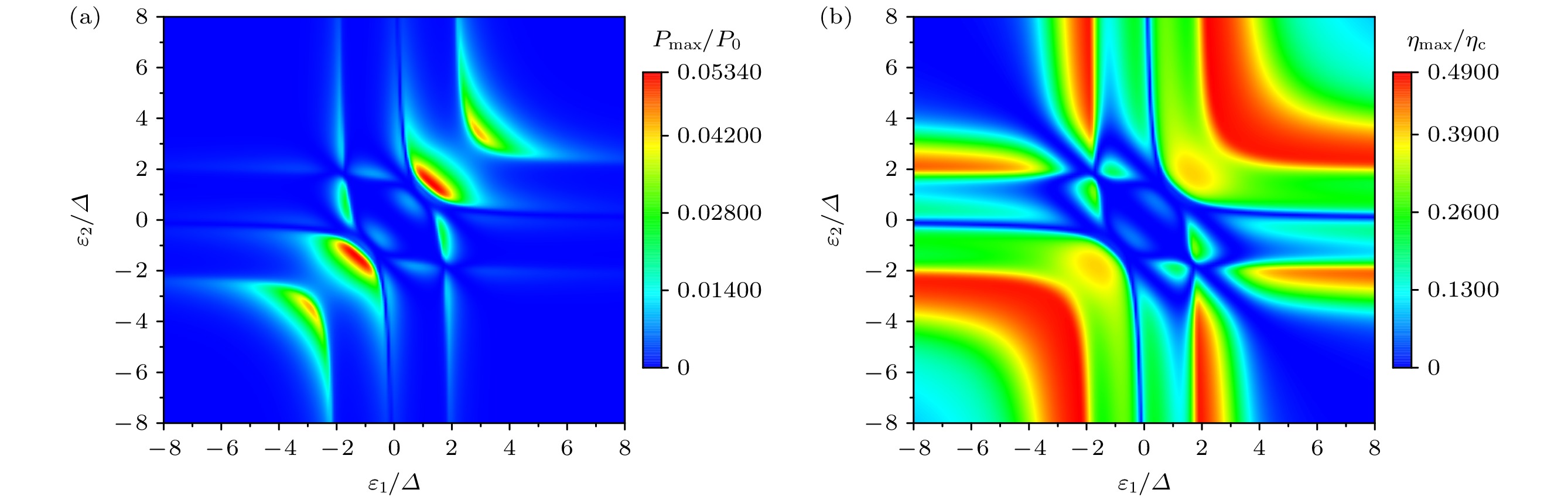
图 7 (a)最大功率
$P_{{\mathrm{max}}}$ (以$P_{0}=(k_{{\mathrm{B}}}\varDelta T)^{2}/h$ 为单位)和(b)最大功率时的效率$\eta_{{\mathrm{max}}P}$ (以卡诺效率$\eta_{{\mathrm{c}}}$ 为单位) 作为量子点能级$\varepsilon_{1}$ 与$\varepsilon_{2}$ 的函数, 其他参数为$\alpha=0.2\varDelta$ ,$\varDelta_{z}=\varDelta$ ,$k_{{\mathrm{B}}}T=0.3\varDelta$ 以及$\theta=\pi/2$ Figure 7. (a) Maximum power
$P_{{\mathrm{max}}}$ (in units of$P_{0}=(k_{{\mathrm{B}}}\varDelta T)^{2}/h$ ) and (b) efficiency at maximum power$ \eta_{{\mathrm{max}}P}$ (in units of Carnot efficiency$\eta_{{\mathrm{c}}}$ ) as a function of the quantum dot’s levels$\varepsilon_{1}$ and$\varepsilon_{2}$ ; the other parameters are$\alpha=0.2\varDelta$ ,$\varDelta_{z}=\varDelta$ ,$k_{{\mathrm{B}}}T=0.3\varDelta$ and$\theta=\pi/2$ . -
[1] 陈晓彬, 段文晖 2015 物理学报 64 186302 doi: 10.7498/aps.64.186302 Chen X B, Duan W H 2015 Acta Phys. Sin. 64 186302 doi: 10.7498/aps.64.186302 [2] Mahan G D, Sofo J O 1996 Proc. Natl. Acad. Sci. USA 93 7436 doi: 10.1073/pnas.93.15.7436 [3] Liu J, Sun Q F, Xie X C 2010 Phys. Rev. B 81 245323 doi: 10.1103/PhysRevB.81.245323 [4] Swirkowicz R, Wierzbicki M, Barnas J 2009 Phys. Rev. B 80 195409 doi: 10.1103/PhysRevB.80.195409 [5] Mazal Y, Meir Y, Dubi Y 2019 Phys. Rev. B 99 075433 doi: 10.1103/PhysRevB.99.075433 [6] Chida K, Fujiwara A, Nishiguchi K 2022 Appl. Phys. Lett. 121 183501 doi: 10.1063/5.0114584 [7] Sanduleac I, Pflaum J, Casian A 2019 J. Appl. Phys. 126 175501 doi: 10.1063/1.5120461 [8] Gomes T C S C, Marchal N, Araujo F A, Piraux L 2019 Appl. Phys. Lett. 115 242402 doi: 10.1063/1.5130718 [9] Wierzbicki M, Swirkowicz R 2010 J. Phys.: Condens. Matter 22 185302 doi: 10.1088/0953-8984/22/18/185302 [10] Wang R Q, Shen L, Shen R, Wang B G, Xing D Y 2010 Phys. Rev. Lett. 105 057202 doi: 10.1103/PhysRevLett.105.057202 [11] Bao W S, Liu Y S, Lei X L 2010 J. Phys.: Condens. Matter 22 315502 doi: 10.1088/0953-8984/22/31/315502 [12] Ghawri B, Mahapatra P S, Garg M, Mandal S, Jayaraman A, Watanabe K, Taniguchi T, Jain M, Chandni U, Ghosh A 2024 Phys. Rev. B 109 045436 doi: 10.1103/PhysRevB.109.045436 [13] Anderson L E, Laitinen A, Zimmerman A, Werkmeister T, Shackleton H, Kruchkov A, Taniguchi T, Watanabe K, Sachdev S, Kim P 2024 Phys. Rev. Lett. 132 246502 doi: 10.1103/PhysRevLett.132.246502 [14] Li J, Niquet Y M, Delerue C 2023 Phys. Rev. B 107 245417 doi: 10.1103/PhysRevB.107.245417 [15] Xu Y, Gan Z X, Zhang S C 2014 Phys. Rev. Lett. 112 226801 doi: 10.1103/PhysRevLett.112.226801 [16] Blasi G, Taddei F, Arrachea L, Carrega M, Braggio A 2020 Phys. Rev. Lett. 124 227701 doi: 10.1103/PhysRevLett.124.227701 [17] Sebastian Bergeret F, Silaev M, Virtanen P, Heikkilä T T 2018 Rev. Mod. Phys. 90 041001 doi: 10.1103/RevModPhys.90.041001 [18] Hwang S Y, Lopez R, Sanchez D 2016 Phys. Rev. B 94 054506 doi: 10.1103/PhysRevB.94.054506 [19] Hwang S Y, Sanchez D, Lopez R 2016 New. J. Phys. 18 093024 doi: 10.1088/1367-2630/18/9/093024 [20] Trocha P, Barnas J 2017 Phys. Rev. B 95 165439 doi: 10.1103/PhysRevB.95.165439 [21] Michaek G, Urbaniak M, Bulka B R, Domanski T, Wysokinski K I 2016 Phys. Rev. B 93 235440 doi: 10.1103/PhysRevB.93.235440 [22] Dutta P, Alves K R, Black-Schaffer A M 2020 Phys. Rev. B 102 094513 doi: 10.1103/PhysRevB.102.094513 [23] Linder J, Balatsky A V 2019 Rev. Mod. Phys. 91 045005 doi: 10.1103/RevModPhys.91.045005 [24] Kubala B, Konig J 2002 Phys. Rev. B 65 245301 doi: 10.1103/PhysRevB.65.245301 [25] Chi F, Li S S 2006 J. Appl. Phys. 100 113703 doi: 10.1063/1.2365379 [26] Kang K, Cho S Y 2004 J. Phys.: Condens. Matter 16 117 doi: 10.1088/0953-8984/16/1/011 [27] Lu H Z, Lü R, Zhu B F 2005 Phys. Rev. B 71 235320 doi: 10.1103/PhysRevB.71.235320 [28] Kubo T, Tokura Y, Tarucha S 2011 Phys. Rev. B 83 115310 doi: 10.1103/PhysRevB.83.115310 [29] Pan H, Lin T H 2006 Phys. Rev. B 74 235312 doi: 10.1103/PhysRevB.74.235312 [30] Bordoloi A, Zannier V, Sorba L, Schrnenberger C, Baumgartner A 2020 Commun. Phys. 3 135 doi: 10.1038/s42005-020-00405-2 [31] Bittermann L, Dominguez F, Recher P 2024 Phys. Rev. B 110 045429 doi: 10.1103/PhysRevB.110.045429 [32] Bułka B R 2022 Phys. Rev. B 106 085424 doi: 10.1103/PhysRevB.106.085424 [33] Yao H, Zhang C, Li Z J, Nie Y H, Niu P B 2018 J. Phys. D: Appl. Phys. 51 175301 doi: 10.1088/1361-6463/aab6e4 [34] Bai L, Zhang L, Tang F R, Zhang R 2023 J. Appl. Phys. 134 184304 doi: 10.1063/5.0172000 [35] Hussein R, Governale M, Sigmund Kohler S, Belzig W, Giazotto F, Alessandro Braggio A 2019 Phys. Rev. B 99 075429 doi: 10.1103/PhysRevB.99.075429 [36] Tabatabaei S M, Sánchez D, Yeyati A L, Sánchez R 2022 Phys. Rev. B 106 115419 doi: 10.1103/PhysRevB.106.115419 [37] Sánchez R, Burset P, Yeyati A L 2018 Phys. Rev. B 98 241414 doi: 10.1103/PhysRevB.98.241414 [38] Gresta D, Real M, Arrachea L 2019 Phys. Rev. Lett. 123 186801 doi: 10.1103/PhysRevLett.123.186801 -
计量
- 文章访问数: 935
- HTML全文浏览数: 935
- PDF下载数: 6
- 施引文献: 0