
 首页
首页 登录
登录 注册
注册


 下载:
下载:
-
黏弹性非牛顿流体在石油化工、生物医药和食品工程等领域具有广泛的应用, 其黏弹性参数直接影响流体流动、传热和传质[1]. 获取非牛顿流体在较宽的剪切频率范围的黏弹性性质是流程装备设计和优化的基础[2,3]. 传统的旋转法由于剪切热等影响, 剪切频率往往在100 Hz以下, 限制了更高剪切频率的研究[4]. 考虑到非牛顿流体气液相界面处由于体相中分子的热运动会激发出振幅为纳米级、波长为微米级的表面波[5], 可以用于施加MHz及以下级别的高频剪切, 因此可以将传统应用于牛顿流体的表面光散射法引入到非牛顿流体黏弹性性质测量, 实现宽频范围内黏弹性的研究. 当激光入射至流体相界面时, 考虑到表面波对于激光的扰动是微弱的, 根据线性响应理论[6], 表面波的色散规律与被其散射的激光, 即散射光的色散规律相同, 因此可以通过研究散射光频谱来研究表面波的功率谱. 当构建起黏弹性非牛顿流体表面波的色散方程及其功率谱, 就可以用于拟合由表面光散射法获得的实验功率谱, 获得宽频剪切条件下的黏弹性. 黏弹性非牛顿流体具有与频率相关的复黏度[7], 因此需要建立合适的复黏度模型来表征其复杂行为, 同时应建立新的色散方程. Harden等(1990)[8]构建了非牛顿流体表面波理论, 预测了非牛顿流体表面波中存在的特征模式. Ohmasa等[9,10]首次提出体相剪切模式, 并通过简单Maxwell模型分析了非牛顿黏弹性流体的色散关系以及频谱特征. Cao等[11]以及 Meunier[12]均在实验中发现了单个应力松弛时间τ, 不足以描述黏弹性非牛顿流体的复杂行为.
因此, 本文尝试通过耦合系列应力松弛时间改进Maxwell模型, 着重分析了表面波的色散规律及其频谱响应特性, 从理论上分析了引入多个应力松弛时间对于色散方程在复平面根的数量和性质的影响, 并通过研究复数根的性态来分析不同类型表面波的存在条件以及对于功率谱的贡献.
-
为了扩展频率反馈模型的适用范围, 本文尝试引入Meunier[12]提出的多个应力松弛时间τ, 可以将上述复黏度模型改进为
式中, τ为应力松弛时间; η1/τ表示高频剪切模量;
${\eta _\infty }$ 为常数项, 可以用来表示高频黏度响应; ω为表面波圆频率; τn = τ/n2, n取1, 2, 3 ···. 当$\omega \tau \ll 1 $ 或者${\eta _1}$ = 0时, 复黏度$\eta (\omega )$ 退化为牛顿流体的黏度表达式. 假设黏弹性非牛顿流体填充z < 0的空间, 并且其表面在xy平面中延伸. 液体的表面张力和密度分别用σ和ρ表示. 流体表面波的色散方程可表示为[5]式中q为表面波波数,
$m(\omega ) = \sqrt {{q^2} - {\text{i}}\omega \rho /\eta (\omega )} $ 为复数,$ m(\omega ) $ 的实部必须为正数, 表示沿$ z $ 方向表面波由界面相向体相的渗透深度[13]. 定义无量纲数Y:式中η为牛顿流体黏度, g为重力加速度. 即Y = (驱动力×惯性力)/(阻尼力)2. 其中驱动力包括表面力和重力, 对于表面波, 表面力远远大于重力, 可以忽略重力的影响. 牛顿流体表面波包含过阻尼模式(Y ≤ 0.145)和毛细波模式(Y > 0.145), 即两种振荡形式转变的临界振荡点由Y决定[14].
根据线性响应理论, 若激光等外源作用对于液体表面波动的扰动是微弱的, 则可以利用表面波对于微弱扰动的反馈计算其功率谱, 功率谱表达式为[15–18]
kB为玻尔兹曼常数, kB = 1.380649 × 10⁻²³ J/K; T为开尔文温度; Im[·]为取虚部函数. 同时, 假设黏度的低频极限为
${\eta _0}$ ,${\eta _0}$ 可以表示为参考Ohmasa方法定义下述无量纲变量[10]:
分别给出当n = 1, 2, 3, 4时的复黏度
$\eta (\omega )$ 无量纲表达式:因此复黏度表达式可以简化为
$\eta (\omega ) = {\eta _0}\dfrac{{g(\overline \omega )}}{{f(\overline \omega )}}$ , 同时定义下列含$\overline \omega $ 的多项式函数:使用上述无量纲变量以及多项式函数[10], 功率谱
${P_{\text{T}}}(q, \omega )$ 可以表示为色散关系可以由多项式方程表示为
该方程可用数值方法求解, 根表示为
${\overline \omega _i} = {\overline \varOmega _i} - {\text{i}}{\overline \varGamma _i}$ , 当实部${\overline \varOmega _i}$ 不为0时, 存在负的共轭根${\overline \omega _i}'= - {\overline \varOmega _i} - {\text{i}}{\overline \varGamma _i}$ . 令$ h(\overline{\omega}) $ 表示方程分子与分母的公因式项, 因此多项式方程可以表达为式中,
${B_n}$ 表示$h(\overline \omega ){\overline \omega ^n}$ 的系数. 利用部分分式展开法[10]可将功率谱${P_{\text{T}}}(q, \omega )$ 表示为式中
${P^i}(q, \omega )$ 为其中
${a_i} = \displaystyle\prod\limits_{j = 1}^n {\dfrac{1}{{{{\overline \omega }_i} - {{\overline \omega }_j}}}} $ $(i \ne j)$ ,$\overline m'(\overline \omega )$ 为$\overline m(\overline \omega )$ 的实部,$\overline m''(\overline \omega )$ 为$\overline m(\overline \omega )$ 的虚部. -
如图1所示, 通过调整应力松弛时间τ的数量n和无量纲应力松弛时间
$\overline \tau $ 的值, 可得到色散方程$ F({\overline \omega _i})\overline m({\overline \omega _i}) + G({\overline \omega _i}) = 0 $ 的根${\overline \omega _i} = {\overline \varOmega _i} - {\text{i}}{\overline \varGamma _i}$ 随无量纲表面张力$\overline \sigma $ 的变化情况.当
$\overline \tau = 0.1$ 时, 弹性模量相对较小, 此时流体与牛顿流体类似, 实际上, (3)式往往可以忽略重力, 因此Y即为无量纲表面张力$ \overline \sigma $ , 根随$\overline \sigma $ 的变化情况也与牛顿流体根的变化趋势一致[13]. 由图1可知,$\overline \sigma $ 大于某临界值时根的表现形式为${\overline \omega _{\text{c}}} = {\overline \varOmega _{\text{c}}} - {\text{i}}{\overline \varGamma _{\text{c}}}$ ; 小于该临界值, 表现为两个纯虚数根$ {\overline \varGamma _{\text{s}}} $ 和${\overline \varGamma _{\text{f}}}$ , n分别为2, 3, 4时, 临界值分别是0.241, 0.287, 0.313. 临界点表征了表面波在特定条件下传播形式发生突变, 小于该值时表面波以两个不同的弛豫时间(${\overline \tau _{\text{s}}} = \overline \varGamma _{\text{s}}^{ - 1}$ 和${\overline \tau _{\text{f}}} = \overline \varGamma _{\text{f}}^{ - 1}$ 分别表示慢波和快波)衰减[9,19]. 由于表面波呈指数衰减, 所以在实验中很难观察到快波. 大于临界值时, 根${\overline \omega _{\text{c}}} = {\overline \varOmega _{\text{c}}} - {\text{i}}{\overline \varGamma _{\text{c}}}$ 的实部${\overline \varOmega _{\text{c}}}$ 随$\overline \sigma $ 增大而增大, 此时恢复力为表面力, 表现出与牛顿流体类似的表面波特征, 即毛细波. 但与牛顿流体不同, 临界值的大小会随着τ和n的增大而增大, 即此时流体仍表现出非牛顿特性. 此外, 会产生与n个数相同的纯虚数根(如图1中的${\overline \varGamma _1}$ ,${\overline \varGamma _2}$ ,${\overline \varGamma _3}$ 和${\overline \varGamma _4}$ ), 并且${\overline \varGamma _i}$ 的大小始终趋近于${n^2}{\overline \tau ^{ - 1}}$ , 即阻尼率仅仅由复黏度的应力松弛时间的倒数决定, 这与具有黏弹性松弛特征的过阻尼模式相对应[20]. 过阻尼模式对应力松弛时间分布敏感, 因此需要引入多个应力松弛时间以描述其弛豫振荡特性[21]. 过阻尼模式仅由应力松弛时间决定, 不同的n对应的应力松弛时间分别与溶剂中的黏性耗散以及聚合物扩散引起的过阻尼模式相对应[8].当
$\overline \tau $ 增大, 弹性模量增大, 弹性行为突出. 如图2所示, 临界点消失, 转变为临界振荡区, 对应图中两条竖直虚线所围成的区域. 振荡区左侧, 原本对应慢波和快波的根$ {\overline \varGamma _{\text{s}}} $ 和${\overline \varGamma _{\text{f}}}$ 消失, 由根${\overline \omega _{\text{r}}} = {\overline \varOmega _{\text{r}}} - {\text{i}}{\overline \varGamma _{\text{r}}}$ 代替. 由图2可知, 根${\overline \omega _{\text{r}}} = {\overline \varOmega _{\text{r}}} - {\text{i}}{\overline \varGamma _{\text{r}}}$ 的实部${\overline \varOmega _{\text{r}}}$ 和虚部${\overline \varGamma _{\text{r}}}$ 均不随$\overline \sigma $ 变化, 只随$\overline \tau $ 改变, 表明此时恢复力不是表面张力, 对应由弹性模量影响的弹性波[22]. 振荡区右侧依旧对应毛细波特征. 因此, 黏弹性非牛顿流体除了具有和牛顿流体类似的过阻尼模式和毛细波模式, 还具有弹性波模式.随着参数
$ \overline \sigma $ 和$ \overline \tau $ 的变化, 色散方程$ G({\overline \omega _i}) \;+ F({\overline \omega _i})\overline m({\overline \omega _i}) = 0 $ 对应振荡衰减形式的根${\overline \omega _i} ={\overline \varOmega _i} \;- {\text{i}}{\overline \varGamma _i}$ 会消失, 而纯虚数根一直存在且为定值, 因此可以推测在功率谱中仅应出现过阻尼模式曲线, 但实际功率谱中却仍存在峰, 表明表面波是传播的. 由于构建色散方程时, 求解过程引入复数平方根$\overline m(\overline \omega ) = {q^{ - 1}}\sqrt {{q^2} - {\text{i}}\omega \rho /\eta (\omega )} $ , 这个复数存在一对共轭值, 使得色散方程$ G({\overline \omega _i}) + F({\overline \omega _i})\overline m({\overline \omega _i}) = 0 $ 和共轭方程$ G({\overline \omega _i}) - F({\overline \omega _i})\overline m({\overline \omega _i}) = 0 $ 分别在复平面的极点和分支切割存在非纯虚数的复数解, 对应传播的表面波或振荡衰减的根[23]. 当考虑体相耗散效应后, 在色散方程基础上引入功率谱方程, 才能同时考虑共轭方程, 因此图2中由于仅考虑色散方程, 在某些区域出现振荡衰减根的中断. 可见, 采用功率谱方程才能完整地描述表面波的特性.临界振荡区及附近会发生严重的耗散现象, 且随
$\overline \tau $ 增大该区域范围也一同扩大, 且会向低$\overline \sigma $ 区移动, 此时仅靠色散方程不足以分析表面波的特征, 需要转换到频域中去分析. 此外, 当n增大时, 对应着聚合物溶液中分子在空间中的扩散与缠结引起的过阻尼模式增多, 弛豫模式增多, 且当增大n时临界振荡区范围也减小. -
改变n,
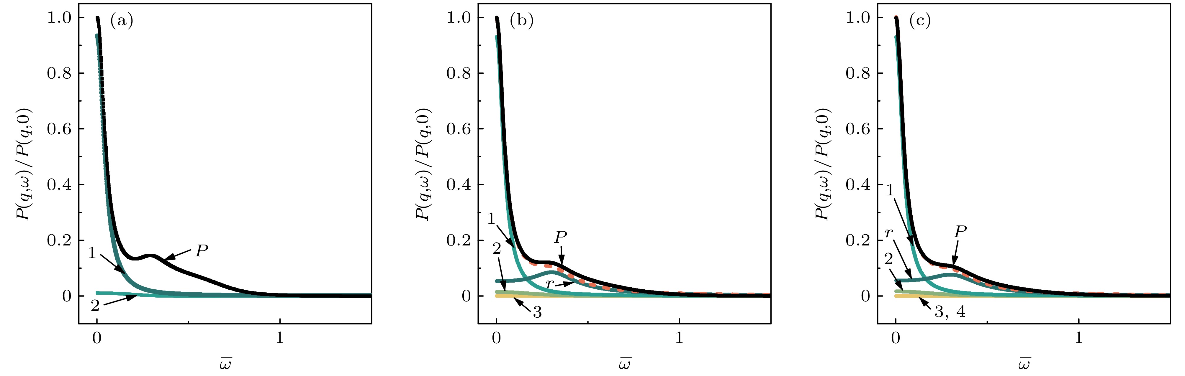
$\overline \sigma $ 和$\overline \tau $ 的值可以得到不同条件下的功率谱, 并且由于复黏度与频率相关, 在黏弹性非牛顿流体中可观察到与简单液体不同的表面波模式. 通过部分分式展开法将总功率谱分解为色散方程根的显式表达. 图中编号与第3节编号的下标对应. 图中1′—4′表示共轭项根所对应谱线; P表示功率谱${P_{\text{T}}}(q, \omega )$ 谱线; c, r分别对应毛细波和弹性波谱线; 1—4对应纯虚数根${\overline \varGamma _i}$ 代表的过阻尼模式.在
$\overline \tau $ 较小时, 聚合物网络的弹性很小近似于简单牛顿流体, 表现出毛细波特征[20]. 如图3所示, 此时τ的个数n对功率谱形状几乎没有影响, 但n的数量也会改变相同参数下功率谱峰值的大小, 对应于不同类型的黏弹性非牛顿流体.图4和图5表示了不同
$\overline \tau $ 值下临界振荡区的功率谱, 均显示了峰特征, 表明体相耗散的影响可以通过功率谱呈现, 并且发现了3种模式共存的现象. 但实际中无法将总功率谱分解为色散方程$F({\overline \omega _i})\overline m({\overline \omega _i}) + G({\overline \omega _i}) = 0$ 的根的显式表达, 需要将共轭项$F({\overline \omega _i})\overline m({\overline \omega _i}) - G({\overline \omega _i}) = 0$ 的根代入计算[10], 即将功率谱有理化, 才可以展现出如图所示的毛细波谱线c和弹性波谱线r.值得注意的是, 这样的考虑只适用于临界振荡区附近的功率谱分解. 这是因为功率谱的有理化并未引入新的信息. 此外, 分解出来的一些曲线无明确的物理意义, 因为共轭项的根全为振荡衰减形式根, 即
$\overline \varOmega i$ 不为0, 但对应曲线却未出现峰. 另外, 在相同参数下随着n的增大, 弹性波和过阻尼模式在毛细波减弱时增强, n的数值能够反映出聚合物网络的黏弹性. 此外, 当n增大时, 毛细波峰值减小, 表面张力恢复作用减弱, n值的不同可以体现不同的黏弹性效果, 对应着不同频率反馈特性的黏弹性非牛顿流体.如图6所示, 在n = 2的情况下处于临界振荡区, 表面波的峰无法分解为根的显式表达, 而通过增大n值可以避开此区域. 图中虚线表示分解后的曲线之和, 可以发现n越大, 与总功率谱曲线P越吻合, 效果越好, 且能单独观察到弹性波曲线r的存在. 此时, 功率谱表现出在低频具有黏弹性松弛特征的过阻尼模式和一个具有小强度的弹性波, 这是聚合物黏弹性效应的表现[24,25].
-
本文通过增加应力松弛时间τ的数量n来改进复黏度模型
$\eta (\omega )$ . 通过改变n,$\overline \tau $ ,$\overline \sigma $ 值, 从理论上分析了不同情况下非牛顿黏弹性流体的表面波特征.1)当n增大, 对应色散方程根数量增加, 弛豫模式增加, 表现为低频的过阻尼模式.
2)当
$\overline \tau $ 增大, 会出现临界振荡区, 该区域表面波特征需要通过功率谱进行分析, 而n增大会减小该区域的范围, 甚至完全避开此区域.3)相同参数下, n增大会抑制表面张力的恢复作用, 使得毛细波强度下降, 弹性波强度提高, n个数的差异能体现聚合物网络的黏弹性差异.
4)不同的n值对应不同的黏弹性效果, 采取合适的n值, 得到合适的弛豫模式, 可以对应不同的黏弹性非牛顿流体.
黏弹性非牛顿流体的表面波色散方程
Surface wave dispersion equations for viscoelastic non-Newtonian fluids
-
摘要: 黏弹性非牛顿流体表面波色散方程研究是开展表面光散射法测量黏弹性等热物性参数的基础. 区别于牛顿流体, 非牛顿体系的复黏度表现出与频率和应力松弛时间相关的非线性特性, 因此建立能够准确描述其复黏度特性的本构模型至关重要. 基于多弛豫时间Maxwell模型, 本文通过总功率谱的模式分解方法构建了表面波色散方程的显式解, 系统考察了弛豫时间参数对表面波模式分布的影响. 本文研究揭示了本构模型中弛豫时间参数数目与体系非线性响应能力的定量关联, 为精确解析非牛顿流体表面波特性提供了依据, 也为表面光散射法黏弹性流体热物理性质测量奠定了理论基础.Abstract:
The study of surface wave dispersion equations in viscoelastic non-Newtonian fluids is the foundation for characterizing the thermophysical properties by using surface light scattering techniques. Unlike Newtonian fluids, non-Newtonian systems have the complex viscosity with nonlinear frequency behavior and stress relaxation time-dependent behavior. Consequently, the development of constitutive models capable of accurately capturing these complex viscosity characteristics is critical. Based on the multi-relaxation-time Maxwell framework, this work establishes a method of explicitly solving the surface wave dispersion equation through modal decomposition of the total power spectrum, which can systematically analyze the influence of relaxation time parameters on surface wave mode distributions. This study quantitatively correlates the number of relaxation time parameters in the constitutive model with the nonlinear response capacity of the system. These findings provide a theoretical foundation for precisely determining the surface wave characteristics in non-Newtonian fluids and advance the application of surface light scattering method to the measurement of thermophysical properties in viscoelastic fluid systems. Based on a multi-relaxation-time Maxwell model, the complex viscosity is formulated by combining multiple stress relaxation time. Utilizing non-depersonalization and polynomial decomposition, we derive the governing equations for surface wave dispersion and the associated power spectrum. By systematically varying the parameter n and dimensionless variables, the roots of the dispersion equations are analyzed to study surface wave modes—including capillary, elastic waves, and overdamped modes—and their spectral signatures. A partial fraction expansion method is employed to decouple the total power spectrum into explicit modal contributions. This method demonstrates how the relaxation parameters determine the distribution of surface wave modes, thereby clarifying the inherent multimodal relaxation dynamics of complex fluids. The proposed framework extends the classical Maxwell model by integrating multiple relaxation times, with a focus on surface wave dispersion behavior and spectral response. Theoretically, it quantifies the influence of relaxation time on the number and topological properties of roots in the complex plane. Furthermore, by correlating the dynamic behaviors of these roots with physical constraints, this study establishes criteria for the existence of different surface wave modes and evaluates their relative contributions to the power spectrum. When the elastic modulus is low and approaches Newtonian fluid behavior, increasing the number of relaxation time parameters n will increase the critical threshold for surface wave mode transition. This simultaneously generates n purely imaginary roots corresponding to overdamped modes. At higher elastic modulus, the critical threshold vanishes and is replaced by an oscillation-dominated regime requiring power spectrum analysis to solve surface wave dynamics problems. Larger n values reduce the spatial extent of this oscillatory regime. In systems with low elastic modulus, n mainly modulates the peak amplitudes in the power spectrum rather than changing its overall shape. Near the oscillation region, the power spectrum clearly distinguishes the contributions from capillary waves, elastic waves, and overdamped modes. Increasing n can enhance the strengths of elasticity and overdamped mode while suppressing the dominance of capillary wave. By incorporating additional relaxation time, the model gains enhance the resolution of multimodal relaxation dynamics, enabling precise characterization of viscoelasticity in complex non-Newtonian fluids. We improve the complex viscosity model by increasing the number of stress relaxation time parameters n. Through the theoretical analysis of parameter variations under different conditions, the surface wave characteristics of non-Newtonian viscoelastic fluids are systematically investigated. The main conclusions are shown below. First, increasing the number of relaxation time parameters n will increase the number of roots in the dispersion equation, introducing additional relaxation modes manifested as low-frequency overdamped behavior. Second, increasing stress relaxation time τ will induce a critical oscillation regime, at which point power spectrum analysis is required for surface wave dynamics. Increasing n can reduce the spatial extent of this regime or even enables its complete avoidance. Third, under identical parameters, higher n suppresses surface tension-driven capillary wave intensity while enhancing elastic wave dominance. Variations in n quantitatively reflect the viscoelastic heterogeneity of polymer networks. Fourth, selecting appropriate n values can tailor the ability of model to resolve specific relaxation modes, making it suitable for different viscoelastic non-Newtonian fluids. -

-
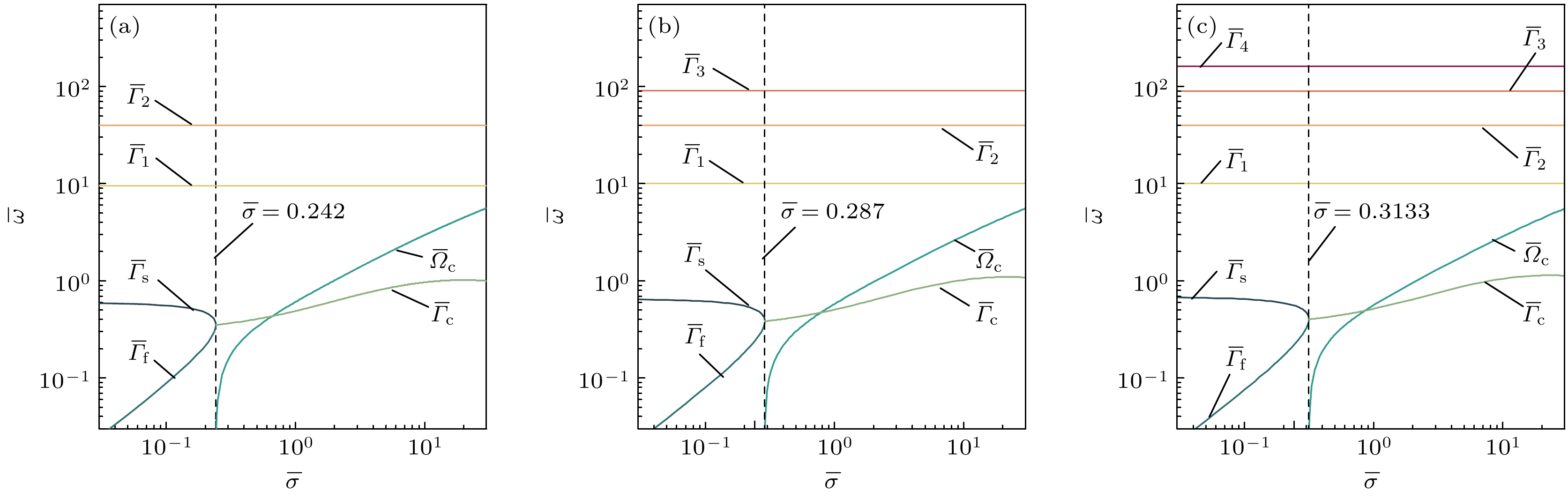
图 1
$\overline \tau $ = 0.1时, 不同n下色散方程的解与$\overline \sigma $ 关系 (a) n = 2; (b) n = 3; (c) n = 4; 其中${\overline \varOmega _{\text{c}}}$ 表示毛细波c的无量纲频率,${\overline \varGamma _{\text{c}}}$ 表示毛细波c的无量纲阻尼率,$ {\overline \varGamma _{\text{s}}} $ 表示慢波s的无量纲阻尼率,${\overline \varGamma _{\text{f}}}$ 表示快波f的无量纲阻尼率,${\overline \varGamma _1}$ —${\overline \varGamma _4}$ 表示纯虚数根Figure 1. Solution of the dispersion equation as a function of
$\overline \sigma $ for different values of n: (a) n = 2; (b) n = 3; (c) n = 4; where${\overline \varOmega _{\text{c}}}$ represents the dimensionless frequency of capillary wave c,${\overline \varGamma _{\text{c}}}$ represents the dimensionless damping rate of capillary wave c,$ {\overline \varGamma _{\text{s}}} $ represents the dimensionless damping rate of slow wave s,${\overline \varGamma _{\text{f}}}$ represents the dimensionless damping rate of fast wave f,${\overline \varGamma _1}$ –${\overline \varGamma _4}$ represent the pure imaginary root.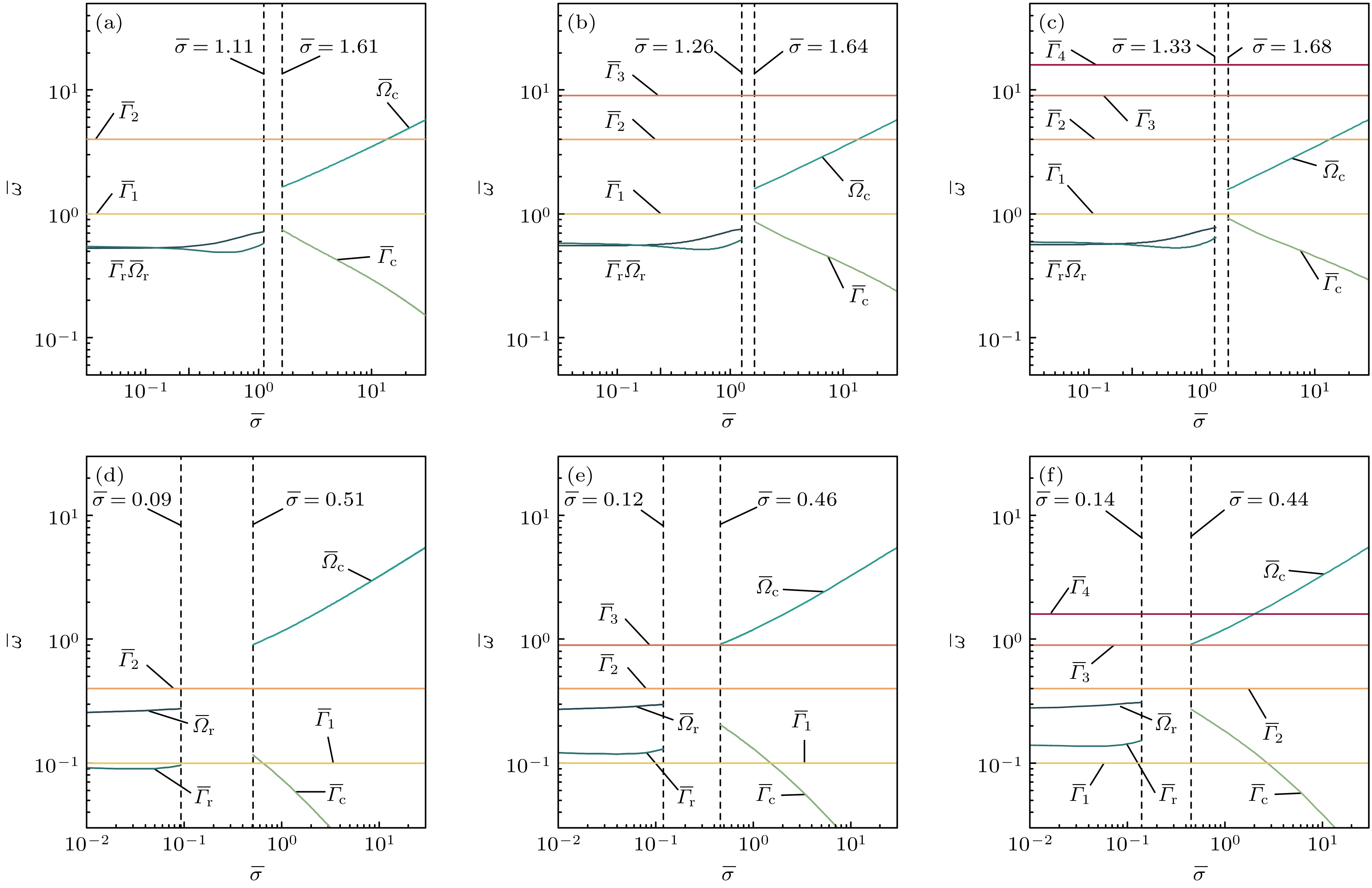
图 2
$\overline \tau $ = 1.0和10.0时, 不同n下色散方程的解与$\overline \sigma $ 的关系 (a) n = 2,$\overline \tau $ = 1.0; (b) n = 3,$\overline \tau $ = 1.0; (c) n = 4,$\overline \tau $ = 1.0; (d) n = 2,$\overline \tau $ = 10.0; (e) n = 3,$\overline \tau $ = 10.0; (f) n = 4,$\overline \tau $ = 10.0; 其中${\overline \varOmega _{\text{r}}}$ 表示毛细波r的无量纲频率,${\overline \varGamma _{\text{r}}}$ 表示毛细波r的无量纲阻尼率Figure 2. Solution of the dispersion equation as a function of
$\overline \sigma $ for varying parameters: (a) n = 2,$\overline \tau $ = 1.0; (b) n = 3,$\overline \tau $ = 1.0; (c) n = 4,$\overline \tau $ = 1.0; (d) n = 2,$\overline \tau $ = 10.0; (e) n = 3,$\overline \tau $ = 10.0; (f) n = 4,$\overline \tau $ = 10.0; where${\overline \varOmega _{\text{r}}}$ represents the dimensionless frequency of capillary wave r,${\overline \varGamma _{\text{r}}}$ represents the dimensionless damping rate of capillary waver.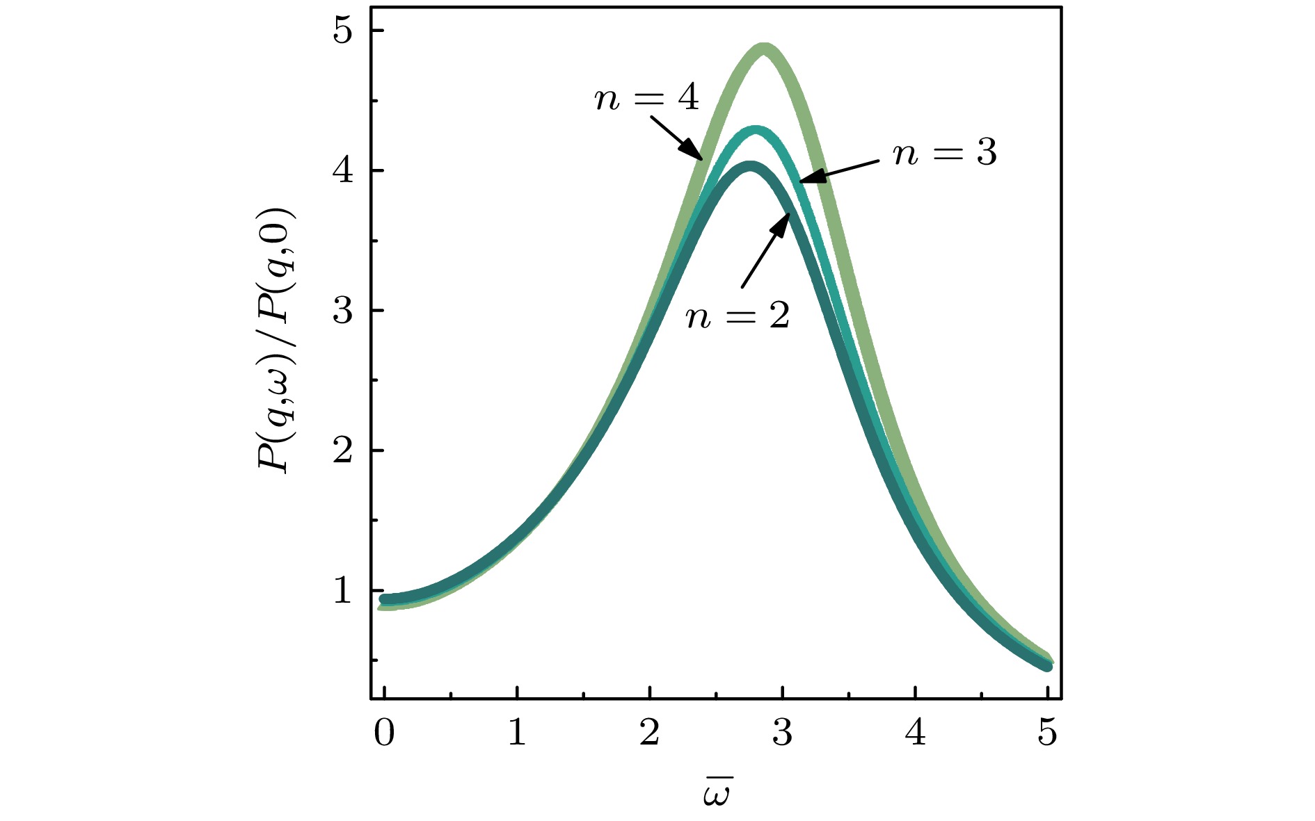
图 3
$\overline \sigma $ = 10.0,$\overline \tau $ = 0.1时, 不同n下的功率谱Figure 3. Power spectrum for various n at
$\overline \sigma $ = 10.0,$\overline \tau $ = 0.1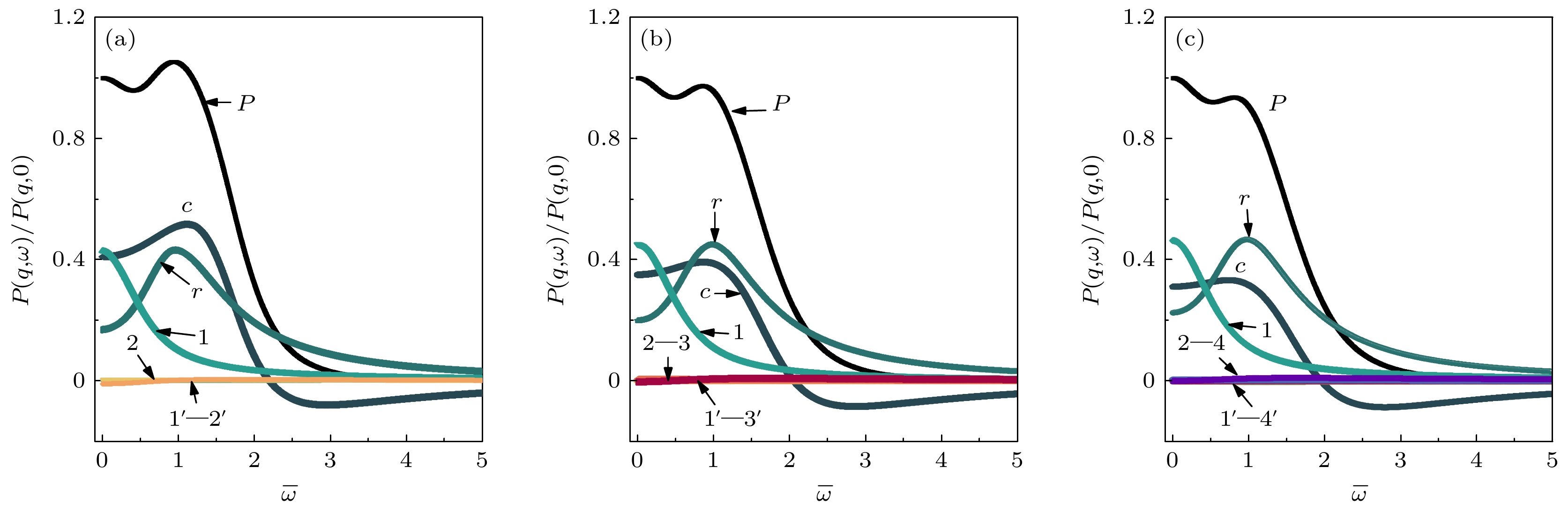
图 4
$\overline \sigma $ = 1.5,$\overline \tau $ = 1.0时, 不同n下的功率谱及其分解 (a) n = 2; (b) n = 3; (c) n = 4Figure 4. Power spectrum and its spectral decomposition for various n at
$\overline \sigma $ = 1.5 and$\overline \tau $ = 1.0: (a) n = 2; (b) n = 3; (c) n = 4.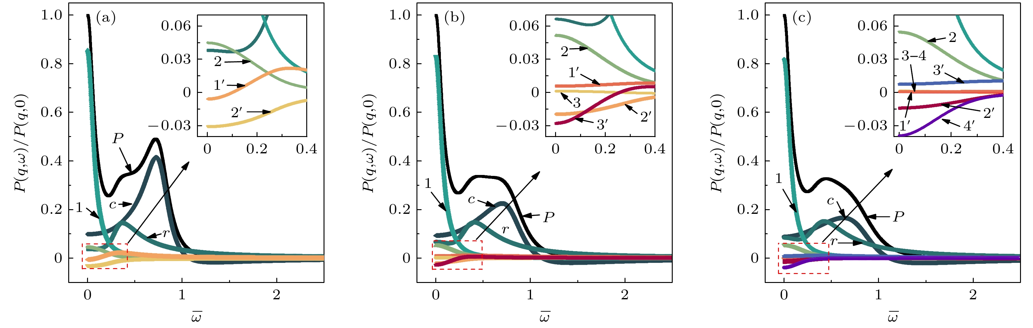
图 5
$\overline \sigma $ = 0.3,$\overline \tau $ = 10.0时, 不同n下的功率谱及其分解 (a) n = 2; (b) n = 3; (c) n = 4Figure 5. Power spectrum and its spectral decomposition for various n at
$\overline \sigma $ = 0.3 and$\overline \tau $ = 10.0: (a) n = 2; (b) n = 3; (c) n = 4. -
[1] Morris B A 2017 The Science and Technology of Flexible Packaging (Oxford, UK: William Andrew) pp121–147 [2] Lanzaro A, Yuan X F 2022 Micromachines 13 256 doi: 10.3390/mi13020256 [3] 刘西洋, 付涛涛, 朱春英, 马友光 2021 化工学报 72 772 doi: 10.11949/0438-1157.20200994 Liu X Y, Fu T T, Zhu C Y, Ma Y G 2021 CIESC J. 72 772 doi: 10.11949/0438-1157.20200994 [4] 邵鸿飞, 高岩立, 任万杰, 李艳玲, 刘元俊, 刘忠民 2019 化学分析计量 28 6 doi: 10.3969/j.issn.1008-6145.2019.01.002 Shao H F, Gao Y L, Ren W J, Li Y L, Liu Y J, Liu Z M 2019 Chem. Anal. Meterage 28 6 doi: 10.3969/j.issn.1008-6145.2019.01.002 [5] Levich V G, Spalding D B 1962 Physicochemical Hydrodynamics (New Jersey: Prentice-Hall) pp591–599 [6] Kadanoff L P, Martin P C 1963 Ann. Phys. 24 419 doi: 10.1016/0003-4916(63)90078-2 [7] Harden J L, Pleiner H, Pincus P A 1989 Langmuir 5 1436 doi: 10.1021/la00090a034 [8] Harden J L, Pleiner H, Pincus P A 1991 J. Chem. Phys. 94 5208 doi: 10.1063/1.460525 [9] Ohmasa Y, Hoshino T, Osada R, Yao M 2009 Phys. Rev. E 79 061601 doi: 10.1103/PhysRevE.79.061601 [10] Ohmasa Y, Yao M 2011 Phys. Rev. E 83 031605 doi: 10.1103/PhysRevE.83.031605 [11] Cao B H, Kim M W, Cummins H Z 1995 J. Chem. Phys. 102 9375 doi: 10.1063/1.468805 [12] Meunier J (edited by Cummins H Z, Pike E R) 2013 Photon Correlation Spectroscopy and Velocimetry (Cham: Springer Science & Business Media) pp515–516 [13] 赵贯甲 2013博士学位论文 (西安: 西安交通大学) Zhao G J 2013 Ph. D. Dissertation (Xi’an: Xi’an Jiaotong University [14] 赵贯甲, 张兴, 尹建国, 马素霞 2022 光学学报 42 2212001 doi: 10.3788/AOS202242.2212001 Zhao G J, Zhang X, Yin J G, Ma S X 2022 Acta Opt. Sin. 42 2212001 doi: 10.3788/AOS202242.2212001 [15] Jäckle J, Kawasaki K 1995 J. Phys. : Condens. Matter 7 4351 doi: 10.1088/0953-8984/7/23/006 [16] Langevin D 1992 Light Scattering by Liquid Surfaces and Complementary Techniques (New York: Marcel Dekker) pp49–51 [17] Kubo R 1966 Rep. Prog. Phys. 29 255 doi: 10.1088/0034-4885/29/1/306 [18] Jäckle J 1998 J. Phys. : Condens. Matter 10 7121 doi: 10.1088/0953-8984/10/32/004 [19] Hoshino T, Ohmasa Y, Osada R, Yao M 2008 Phys. Rev. E 78 061604 doi: 10.1103/PhysRevE.78.061604 [20] Wang C H, Huang Q R 1997 J. Chem. Phys. 107 5898 doi: 10.1063/1.474315 [21] Zang D Y, Zhang Y J 2011 Sci. China Phys. Mech. Astron. 54 1587 doi: 10.1007/s11433-011-4451-5 [22] Dorshow R B, Turkevich L A 1993 Phys. Rev. Lett. 70 2439 doi: 10.1103/PhysRevLett.70.2439 [23] Ablowitz M J, Fokas A S 2003 Complex Variables: Introduction and Applications (Cambridge: Cambridge University Press) pp206–245 [24] Huang Q R, Wang C H, Deng N J 1998 J. Chem. Phys. 108 3827 doi: 10.1063/1.475771 [25] Huang Q R, Wang C H 1998 J. Chem. Phys. 109 6103 doi: 10.1063/1.477237 -
计量
- 文章访问数: 37
- HTML全文浏览数: 37
- PDF下载数: 4
- 施引文献: 0