
 首页
首页 登录
登录 注册
注册


-
钨具有高熔点、高热导率、低热膨胀系数、低溅射率和低燃料滞留率等优点[1], 现有及未来许多核聚变装置如EAST[2], CFETR[3]和ITER[4]均选择钨作为其面向等离子体壁的材料[5,6]. 然而作为高Z元素, 钨杂质在等离子体芯部的聚集会导致能量损失, 不稳定性提高, 甚至引发等离子体破裂[7], 因此亟需研究钨杂质的输运和聚芯[8].
在许多托卡马卡装置的研究中, 研究人员通过改变加热方式结合数值模拟, 探究了钨杂质在不同条件下的芯部输运行为. 杂质输运主要有新经典输运和湍流输运[9], 其中新经典输运表现出对杂质原子序数Z的强烈依赖性[10], 较大的Z会导致较强的新经典输运. 因此对于高Z钨杂质需要研究新经典输运对其聚芯的影响. 已有研究表明, 离子温度梯度会对杂质的新经典输运产生重要影响. EAST实验上通过中性束注入(NBI)[11]和电子回旋共振加热(ECRH)[12]提高电子温度(Te)及其梯度, 有效抑制了钨的新经典对流(neoclassical pinch), 降低芯部钨杂质的密度; 同时, 通过新经典(NEO)和湍流输运(TGLF)模型相结合, 成功预测了钨的新经典对流方向[12]. JET实验上通过离子回旋共振加热(ICRH)同样发现[13], 温度的升高会增强新经典向外对流输运、增强钨的排出, 其趋势与新经典输运模型NEOART预测一致. Lee等[14]使用NEO代码针对KSTAR上钨杂质的输运进行了数值模拟, 研究发现新经典输运中的对流受离子温度梯度影响, 会产生温度屏蔽, 可以减小钨杂质在芯部的聚集. 影响钨杂质新经典输运的另一个因素是环向旋转[15]. Mochinaga等[16]利用集成模拟程序TASK, 模拟研究了JET装置中环向旋转对杂质输运的影响, 发现其通过离心力作用增强了钨的内向输运, 提高了芯部钨杂质浓度. Lim等[17]通过回旋动力学代码(GYSELA)模拟也得到了相似的结果. 这些研究均表明强旋转会增强向内对流, 从而增大钨杂质的芯部密度.
以上研究通过实验及数值模拟均发现, 新经典输运会对钨杂质聚芯产生显著影响, 其中向内的 新经典对流会导致钨杂质向芯部聚集. 然而, 目前对新经典对流各分量的研究相对较少. 托卡马克中背景等离子体参数在径向上的变化将直接影响杂质的新经典对流分量, 不同的碰撞模式也会导致 新经典对流的主导分量发生变化, 从而影响杂质分布. 因此, 需要深入研究新经典对流不同分量对芯部杂质的影响, 从而理解杂质的输运行为及聚芯 控制.
“中国环流三号”(HL-3)是新一代可控核聚变装置[18,19], 未来可能会使用钨作为其面向等离子体壁材料[20–23], 因此需要开展钨杂质的相关研究. 本文围绕HL-3上钨杂质聚芯问题, 使用芯部钨杂质输运程序STRAHL开展数值模拟研究. 主要研究氩气注入条件下新经典输运对钨杂质聚芯的影响, 通过模拟不同新经典输运情况下钨杂质分布, 解释了各对流分量对杂质聚芯的影响, 尤其是Pfirsche-Schlüter (PS)分量对杂质聚芯的抑制机理. 本文第2节详细介绍使用的程序STRAHL[24]、相关程序IMPEDGE[25]和SOLPS-ITER[26], 以及相应的模拟设置. 第3节展示模拟结果, 分析新经典输运对钨杂质聚集的影响, 聚焦于芯部杂质的新经典对流主导分量对杂质输运的作用. 第4节对研究结果进行总结, 并对未来研究进行展望.
-
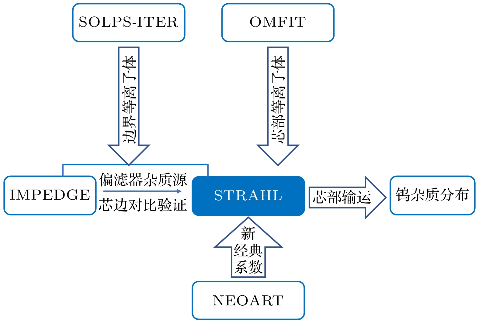
本文主要采用STRAHL程序结合SOLPS-ITER及IMPEDGE开展钨杂质在等离子体芯部的输运和聚集行为模拟研究. 首先, 利用SOLPS-ITER程序模拟边缘背景等离子体参数, 作为输入数据提供给IMPEDGE及STRAHL程序. IMPEDGE计算得到对应的外中平面边界区域钨杂质密度分布. STRAHL程序则结合边缘背景参数以及OMFIT中EFIT[27], ONETWO[28], TGYRO[29]模拟得到的芯部背景参数[30], 通过调节边缘湍流输运系数, 使其模拟的边缘钨杂质分布与IMPEDGE程序的结果一致. 在此基础上, 通过扫描并选取合适的芯部湍流输运系数, 获得在无新经典输运条件的芯部钨杂质分布. 随后, 使用STRAHL子程序NEOART[31]计算得到的新经典输运系数应用于STRAHL模拟中, 进一步得到包含新经典输运的杂质分布. 图1为模拟方法流程图.
STRAHL是一款用于模拟托卡马克芯部杂质径向输运和辐射的程序, 通过求解杂质离子连续性方程, 并结合新经典输运和湍流输运模型, 可模拟杂质在等离子体中的密度分布和能量辐射损失.
对于杂质中性粒子, 假设其以给定均匀径向速度
$ {v}_{0}=-\sqrt{{2{\mathrm{e}}{E}_{0}}/{{m}_{{\mathrm{I}}}}} $ 进入等离子体, 其中$ {E}_{0} $ 表示粒子能量,$ {m}_{{\mathrm{I}}} $ 表示质量, 最终经电离变为离子, 电离源项主要考虑由中性粒子电离为一价离子. 杂质离子输运的连续性方程为[24]其中,
$ {n}_{{\mathrm{I}}, Z} $ 表示价态为Z的I杂质离子密度,$ {Q}_{{\mathrm{I}}, Z} $ 表示碰撞项(包括电离、复合和电荷交换等碰撞),$ {\varGamma }_{{\mathrm{I}}, Z} $ 表示杂质的总径向粒子流密度.碰撞项
$ {Q}_{{\mathrm{I}}, Z} $ 表达式为[24]式中, 等号右侧第1项表示当前电离态(Z)粒子之间的电离、复合和电荷交换碰撞, 第2项表示从前一电离态(
$Z-1 $ )到当前电离态(Z)的电离, 第3项表示从高电离态(Z+1)到当前电离态的复合. 其中,$ {S}_{{\mathrm{I}}, Z} $ 表示电离速率系数,$ {\alpha }_{{\mathrm{I}}, Z} $ 表示辐射复合和双电子复合系数,$ {\alpha }_{{\mathrm{I}}, Z}^{{\mathrm{C}}{\mathrm{X}}} $ 表示电荷交换的复合系数.$ {\varGamma }_{{\mathrm{I}}, Z} $ 包含扩散和对流项, 表达式为[24]每项又包含新经典输运(NEO)和湍流输运(ANO)两个分量. 因此,
$ {\varGamma }_{{\mathrm{I}}, Z} $ 又可使用分量形式表示[32]:其中,
$ {\varGamma }_{{\mathrm{I}}, Z}^{{\mathrm{N}}{\mathrm{E}}{\mathrm{O}}} $ 和$ {\varGamma }_{{\mathrm{I}}, Z}^{{\mathrm{A}}{\mathrm{N}}{\mathrm{O}}} $ 为新经典和湍流输运分量,$ {D}^{{\mathrm{N}}{\mathrm{E}}{\mathrm{O}}} $ 和$ {D}^{{\mathrm{A}}{\mathrm{N}}{\mathrm{O}}} $ 分别为新经典和湍流扩散系数,$ {v}^{{\mathrm{N}}{\mathrm{E}}{\mathrm{O}}} $ 和$ {v}^{{\mathrm{A}}{\mathrm{N}}{\mathrm{O}}} $ 分别是新经典和湍流对流速度,$ {D}^{{\mathrm{T}}{\mathrm{O}}{\mathrm{T}}{\mathrm{A}}{\mathrm{L}}} $ =$ {D}^{{\mathrm{N}}{\mathrm{E}}{\mathrm{O}}} $ +$ {D}^{{\mathrm{A}}{\mathrm{N}}{\mathrm{O}}} $ 为总扩散系数,$ {v}^{{\mathrm{T}}{\mathrm{O}}{\mathrm{T}}{\mathrm{A}}{\mathrm{L}}} $ =$ {v}^{{\mathrm{N}}{\mathrm{E}}{\mathrm{O}}}+{v}^{{\mathrm{A}}{\mathrm{N}}{\mathrm{O}}} $ 为总对流速度. 新经典输运分量$ {\varGamma }_{{\mathrm{I}}, Z}^{{\mathrm{N}}{\mathrm{E}}{\mathrm{O}}} $ 包含3个组成部分, 即PS分量$ {\varGamma }_{{\mathrm{P}}{\mathrm{S}}}^{{\mathrm{N}}{\mathrm{E}}{\mathrm{O}}} $ , 经典分量(classical)$ {\varGamma }_{{\mathrm{C}}{\mathrm{L}}}^{{\mathrm{N}}{\mathrm{E}}{\mathrm{O}}} $ 和香蕉平台分量(banana-plateau)$ {\varGamma }_{{\mathrm{B}}{\mathrm{P}}}^{{\mathrm{N}}{\mathrm{E}}{\mathrm{O}}} $ , 表达式为[33]接下来将对这3个分量进行介绍. PS输运主要源自沿磁场方向的摩擦力, 其会导致粒子在等离子体中发生平行流动, 产生径向分量, 主要发生在具有较高碰撞率的区域, 本工作主要关注PS的径向输运. 经典输运由带电粒子之间的库仑碰撞引起, 库仑碰撞导致粒子径向位移, 从而形成扩散和对流输运, 主要依赖于碰撞频率, 通常发生在高碰撞区域中. 香蕉-平台输运是由俘获粒子沿着磁场的香蕉轨道运动引起, 一般发生在低碰撞区域, 其扩散系数通常远大于经典输运的扩散系数.
为了便于分析, 将(5)式中
$ {\varGamma }_{{\mathrm{I}}, Z}^{{\mathrm{N}}{\mathrm{E}}{\mathrm{O}}} $ 的3个组成部分进一步表达为扩散和对流形式:其中,
$ x $ 表示PS, CL, BP分量,$ D_x^{\mathrm{N}\mathrm{E}\mathrm{O}} $ 和$ {v}_{x}^{{\mathrm{N}}{\mathrm{E}}{\mathrm{O}}} $ 为$ x $ 分量的新经典扩散和对流系数.$ {v}_{x}^{{\mathrm{N}}{\mathrm{E}}{\mathrm{O}}} $ 可以表示为[33]式中,
$ {z}_{{\mathrm{I}}} $ 和$ {z}_{{\mathrm{D}}} $ 分别为杂质和氘离子电荷数,$ {H}_{{\mathrm{X}}} $ 为负的离子温度梯度因子,$ {n}_{{\mathrm{D}}} $ 和$ {T}_{{\mathrm{D}}} $ 分别为氘离子密度和温度. (7)式表明$ {v}_{x}^{{\mathrm{N}}{\mathrm{E}}{\mathrm{O}}} $ 与电荷数ZI成正比, 此外,$ {v}_{x}^{{\mathrm{N}}{\mathrm{E}}{\mathrm{O}}} $ 由离子温度梯度$ {{\mathrm{d}} \ln {T}_{{\mathrm{D}}}}/{{\mathrm{d}}r} $ 和密度梯度${{\mathrm{d}}\ln {n}_{{\mathrm{D}}}}/{{\mathrm{d}}r} $ 共同决定,${{\mathrm{d}} \ln {T}_{{\mathrm{D}}}}/{{\mathrm{d}}r} $ 驱动对流导致杂质从芯部排出,$ {{\mathrm{d}} \ln{n}_{{\mathrm{D}}}}/{{\mathrm{d}}r} $ 驱动对流则引起杂质芯部聚集, 两者相互竞争决定了杂质的对流方向.IMPEDGE是导向中心近似的蒙特卡罗边界杂质输运程序[25], 考虑了钨杂质受到的摩擦力、热力以及反常输运等效应, 作为边界杂质输运程序, 用于提供外中平面钨杂质的径向分布情况. SOLPS-ITER程序[34,35]由二维等离子体流体程序B2.5和三维蒙特卡罗中性粒子输运程序EIRENE 组成, 在本研究中用于为IMPEDGE和STRAHL分别提供背景等离子体.
-
本研究中采用HL-3下单零放电位形, 面向等离子体壁材料为钨, 模拟粒子为燃料氘. 考虑外打击点附近充氩气情况, 利用SOLPS-ITER模拟边界等离子体参数, 其中氩气会影响背景等离子体参数及入射到靶板的能流和粒子流. 流入芯部边界处(core-edge interface, CEI)功率固定为PCEI = 10 MW, 模拟中电子和离子平分. 对应的放电功率为15 MW, 假设芯部区域辐射33%的加热功率. CEI处氘离子密度为nD+, CEI = 6.5×10¹⁹ m–3, 对应的分界线处Te, sep ~ 178 eV, ne, sep ~ 4×10¹⁹ m–3. 模拟中不考虑漂移, 也未追踪溅射的钨杂质, 具体模拟设置可以参考文献[36].
边界钨杂质分布由IMPEDGE模拟得到, 采用SOLPS-ITER提供的背景等离子体数据, 根据物理溅射经验公式[37–39]计算出钨杂质的总侵蚀流为5.48×10²⁰ W·atoms/s, 模拟得到钨杂质的渗透率(进入芯部的粒子数/发射的总粒子数)为~0.043, 因此流入最外封闭磁力线的钨杂质流为2.36×10¹⁹ W·atoms/s. 在IMPEDGE模拟中, 钨杂质源主要是氩杂质离子侵蚀靶板导致. 在STRAHL程序模拟中, 使用IMPEDGE得到的跨越最外封闭磁力的总的钨杂质流作为杂质源项, 设置于LCFS附近.
-
本研究采用数值模拟方法, 探究钨杂质在等离子体芯部的分布, 主要研究新经典输运对钨杂质聚芯的影响. 为研究新经典输运的作用, 首先需要获取背景等离子体参数. 由SOLPS-ITER和OMFIT模拟得到边缘及芯部等离子体参数, 作为IMPEDGE及STRAHL程序的输入参数. 图2(a)为电子密度(ne)分布, 其由边缘至芯部逐渐升高, 在边缘分布陡峭而在芯部逐渐平缓, 芯部最大达
$ 1.3 \times {10}^{20}\;{{\mathrm{m}}}^{-3} $ . 图2(b)为电子温度(Te)分布, 其随径向向内逐渐升高, 芯部最高达8 keV. 图2(c)为离子温度(Ti)信息, 芯部达10 keV. 程序模拟得到边缘及芯部背景参数后, 可以进行后续模拟工作.在此基础上, 结合IMPEDGE与STRAHL模拟, 首先得到无新经典输运情况下的钨杂质密度(
$ {n}_{{\mathrm{W}}}^{{\mathrm{t}}{\mathrm{o}}{\mathrm{t}}} $ )分布. 具体而言, IMPEDGE模拟给出区域$ \rho $ = 0.98—1.01内的$ {n}_{{\mathrm{W}}}^{{\mathrm{t}}{\mathrm{o}}{\mathrm{t}}} $ 分布. 然后, 通过调节STRAHL中的湍流输运系数(包括对流$ {v}^{{\mathrm{A}}{\mathrm{N}}{\mathrm{O}}} $ 、扩散系数$ {D}^{{\mathrm{A}}{\mathrm{N}}{\mathrm{O}}} $ ), 使得边界区域$ {n}_{{\mathrm{W}}}^{{\mathrm{t}}{\mathrm{o}}{\mathrm{t}}} $ 分布与IMPEDGE一致, 如图3(a)所示. 对应的边缘湍流系数分布如图3(b)所示, 其中$ {v}^{{\mathrm{A}}{\mathrm{N}}{\mathrm{O}}} $ 为负值(指向芯部), 最大达$ -120\;{\mathrm{m}}/{\mathrm{s}} $ (绝对值), 并随径向呈现逐渐减小的分布; 湍流扩散为$ {D}^{{\mathrm{A}}{\mathrm{N}}{\mathrm{O}}}=0.3\;{{\mathrm{m}}}^{2}/{\mathrm{s}} $ , 呈均匀分布. 湍流输运系数在STRAHL程序设置中为自定义分布, 其分布趋势和数量级参考文献[40,41]进行设置. 本研究使用的加热功率为15 MW, 对应芯部区域辐射约为5 MW (占比33%). 接下来, 开展芯部($ \rho $ = 0—0.98区域)湍流输运系数扫描, 通过计算芯部辐射, 确定适合的系数, 也即当芯部辐射为5 MW时, 所对应的$ \rho $ = 0—0.98区域的$ {v}^{{\mathrm{A}}{\mathrm{N}}{\mathrm{O}}} $ 和$ {D}^{{\mathrm{A}}{\mathrm{N}}{\mathrm{O}}} $ 为合适的系数, 如图3(c)所示. 可以看到,$ {v}^{{\mathrm{A}}{\mathrm{N}}{\mathrm{O}}} $ 始终为负值会增强钨杂质向内输运, 其绝对值随径向先增大后减小, 表示$ {v}^{{\mathrm{A}}{\mathrm{N}}{\mathrm{O}}} $ 对杂质向内输运的影响先增强后减弱.$ {D}^{{\mathrm{A}}{\mathrm{N}}{\mathrm{O}}} $ 为正值会驱动钨杂质向外扩散, 其随径向增大后逐渐减小, 表明$ {D}^{{\mathrm{A}}{\mathrm{N}}{\mathrm{O}}} $ 先增强后减低杂质向外的扩散. 在湍流输运系数确定之后, 即可模拟获得钨杂质的分布, 并进一步研究影响其分布的主要物理因素.为研究新经典输运对杂质芯部密度的影响, 采用NEOART计算杂质的新经典输运系数(新经典对流和扩散系数), 并将其集成到STRAHL模拟中以得到新经典输运下的钨杂质分布. NEOART中, 计算区域为径向
$ \rho =0—0.9 $ , 而在边缘区域($ \rho > 0.9 $ )由于开放的磁力线和较低的电子温度, NEOART计算不准确, 因此不考虑新经典输运. 本工作主要关注新经典对流的影响, 因此对新经典扩散系数不做过多描述. 图4(a)中展示了$ {v}^{{\mathrm{A}}{\mathrm{N}}{\mathrm{O}}} $ 、新经典对流($ {v}^{{\mathrm{N}}{\mathrm{E}}{\mathrm{O}}} $ )和总对流($ {v}^{{\mathrm{T}}{\mathrm{O}}{\mathrm{T}}{\mathrm{A}}{\mathrm{L}}}={v}^{{\mathrm{A}}{\mathrm{N}}{\mathrm{O}}}+{v}^{{\mathrm{N}}{\mathrm{E}}{\mathrm{O}}} $ )在中平面的径向分布.$ {v}^{{\mathrm{A}}{\mathrm{N}}{\mathrm{O}}} $ 整体呈向内负值, 引起杂质聚集;$ {v}^{{\mathrm{N}}{\mathrm{E}}{\mathrm{O}}} $ 整体上为正值, 仅在深芯部出现负值, 向外新经典对流有助于杂质排出. 然而, 杂质密度的最终分布取决于$ {v}^{{\mathrm{T}}{\mathrm{O}}{\mathrm{T}}{\mathrm{A}}{\mathrm{L}}} $ ,$ {v}^{{\mathrm{N}}{\mathrm{E}}{\mathrm{O}}} $ 与$ {v}^{{\mathrm{A}}{\mathrm{N}}{\mathrm{O}}} $ 的竞争导致区域$ \rho =0.72—0.90 $ 内$ {v}^{{\mathrm{N}}{\mathrm{E}}{\mathrm{O}}} $ 可以完全抵$ {v}^{{\mathrm{A}}{\mathrm{N}}{\mathrm{O}}} $ , 导致$ {v}^{{\mathrm{T}}{\mathrm{O}}{\mathrm{T}}{\mathrm{A}}{\mathrm{L}}} $ 为正, 促进杂质排出. 而进入$ \rho =0.72 $ 后$ {v}^{{\mathrm{N}}{\mathrm{E}}{\mathrm{O}}} $ 不能完全抵消$ {v}^{{\mathrm{A}}{\mathrm{N}}{\mathrm{O}}} $ ,$ {v}^{{\mathrm{T}}{\mathrm{O}}{\mathrm{T}}{\mathrm{A}}{\mathrm{L}}} $ 为负导致杂质向内聚集. 值得注意的是$ \rho =0.72 $ 处是$ {v}^{{\mathrm{T}}{\mathrm{O}}{\mathrm{T}}{\mathrm{A}}{\mathrm{L}}} $ 由正值转为负值的转折点.由于钨杂质的分布是由其在不同区域输运的综合作用决定, 而不同区域的新经典对流的作用不同, 因此需要理解
$ {v}^{{\mathrm{N}}{\mathrm{E}}{\mathrm{O}}} $ 的分布对$ {n}_{{\mathrm{W}}}^{{\mathrm{t}}{\mathrm{o}}{\mathrm{t}}} $ 分布的影响. 为了更加直观展示$ {v}^{{\mathrm{N}}{\mathrm{E}}{\mathrm{O}}} $ 分布的影响, 将径向分为两个区域: 区域一为$ \rho =0.72—0.9 $ , 区域二为$ \rho = 0—0.72 $ . 模拟了3种情况, 分别为无新经典对流(W/O NEO), 仅$ \rho =0.72—0.90 $ 有新经典对流(NEO: 0.72—0.90)和$ \rho =0—0.90 $ 有新经典对流(NEO: 0—0.9), 如图4(b)所示. 通过这3种情况的对比, 可以获得新经典对流分别在两个区域和整体上对于$ {n}_{{\mathrm{W}}}^{{\mathrm{t}}{\mathrm{o}}{\mathrm{t}}} $ 分布的影响.我们通过对比3种情况下的
$ {n}_{{\mathrm{W}}}^{{\mathrm{t}}{\mathrm{o}}{\mathrm{t}}} $ 分布以及两个不同位置($ \rho =0.00 $ 和$ \rho =0.72 $ )处的$ {n}_{{\mathrm{W}}}^{{\mathrm{t}}{\mathrm{o}}{\mathrm{t}}} $ , 以分析其对钨杂质密度分布的具体影响. 图4(c)展示了相应的$ {n}_{{\mathrm{W}}}^{{\mathrm{t}}{\mathrm{o}}{\mathrm{t}}} $ 分布, 表1列出了两个位置处的钨杂质密度($ {n}_{{\mathrm{w}}}^{\rho =0.72} $ 和$ {n}_{{\mathrm{w}}}^{\rho =0} $ ), 以及$ \rho =0 $ 处的钨杂质浓度$ {C}_{{\mathrm{w}}}^{\rho =0} $ 和其导致的总辐射损失密度$ {P}_{{\mathrm{r}}{\mathrm{a}}{\mathrm{d}}}^{\rho =0} $ .无
$ {v}^{{\mathrm{N}}{\mathrm{E}}{\mathrm{O}}} $ 的情况下,$ {n}_{{\mathrm{W}}}^{{\mathrm{t}}{\mathrm{o}}{\mathrm{t}}} $ 由边界至芯部逐渐升高, 在$ \rho =0.72 $ 处$ {n}_{{\mathrm{W}}}^{{\mathrm{t}}{\mathrm{o}}{\mathrm{t}}} $ 为$ 6.0\times {10}^{15}\;{{\mathrm{m}}}^{-3} $ , 在$ \rho =0 $ 处达到最大值$ 1.1\times {10}^{16}\;{{\mathrm{m}}}^{-3} $ , 对应的$ {C}_{{\mathrm{w}}}^{\rho =0} $ =7.70×10⁻⁵, 钨杂质导致的能流辐射损失密度$ {P}_{{\mathrm{r}}{\mathrm{a}}{\mathrm{d}}}^{\rho =0} $ = 0.26 MW/m3. 其中$ \rho =1.01 $ 至$ \rho =0.98 $ 处$ {n}_{{\mathrm{W}}}^{{\mathrm{t}}{\mathrm{o}}{\mathrm{t}}} $ 急剧增大, 这是由于该处较大的$ {v}^{{\mathrm{A}}{\mathrm{N}}{\mathrm{O}}} $ 导致, 见图3(b); 进入$ \rho =0.98 $ 后至芯部$ \rho =0 $ 处$ {n}_{{\mathrm{W}}}^{{\mathrm{t}}{\mathrm{o}}{\mathrm{t}}} $ 增大趋势减缓, 这是因为芯部$ {v}^{{\mathrm{A}}{\mathrm{N}}{\mathrm{O}}} $ 相对边界较小但依旧是负值, 见图3(c).在区域
$ \rho =0.72-0.90 $ 加入$ {v}^{{\mathrm{N}}{\mathrm{E}}{\mathrm{O}}} $ 后,$ \rho =0.90 $ 以外由于无$ {v}^{{\mathrm{N}}{\mathrm{E}}{\mathrm{O}}} $ 的影响,$ {n}_{{\mathrm{W}}}^{{\mathrm{t}}{\mathrm{o}}{\mathrm{t}}} $ 分布相对于无$ {v}^{{\mathrm{N}}{\mathrm{E}}{\mathrm{O}}} $ 情况不发生变化; 但在进入$ \rho =0.72—0.90 $ 区域, 由于向外的$ {v}^{{\mathrm{N}}{\mathrm{E}}{\mathrm{O}}} $ ,$ {n}_{{\mathrm{W}}}^{{\mathrm{t}}{\mathrm{o}}{\mathrm{t}}} $ 显著下降,$ \rho =0.72 $ 处杂质密度从$ 6.0\times {10}^{15}\;{{\mathrm{m}}}^{-3} $ (W/O NEO)降至$ 3.8\times {10}^{15}\;{{\mathrm{m}}}^{-3} $ (With NEO$ \rho $ =0.72—0.90). 进入$ \rho =0.72 $ 后由于无$ {v}^{{\mathrm{N}}{\mathrm{E}}{\mathrm{O}}} $ , 湍流输运主导杂质向内输运,$ {n}_{{\mathrm{W}}}^{{\mathrm{t}}{\mathrm{o}}{\mathrm{t}}} $ 再次上升, 但相比无$ {v}^{{\mathrm{N}}{\mathrm{E}}{\mathrm{O}}} $ 情况,$ \rho =0 $ 处的$ {n}_{{\mathrm{W}}}^{{\mathrm{t}}{\mathrm{o}}{\mathrm{t}}} $ 仍有显著下降, 即由$ 1.1\times {10}^{16}\;{{\mathrm{m}}}^{-3} $ 降至$ 5.8\times {10}^{15}\;{{\mathrm{m}}}^{-3} $ . 浓度从原先的$ {C}_{{\mathrm{w}}}^{\rho =0.00} $ = 7.70×10⁻⁵降至4.20×10⁻⁵, 芯部$ \rho =0 $ 处杂质辐射能量从$ {P}_{{\mathrm{r}}{\mathrm{a}}{\mathrm{d}}}^{\rho =0}=0.26\;{\mathrm{M}}{\mathrm{W}}/ $ m3下降到0.15 MW/m3.在区域
$ \rho =0—0.90 $ 加入$ {v}^{{\mathrm{N}}{\mathrm{E}}{\mathrm{O}}} $ 后, 在$ \rho =0.72— 1.01 $ 区域,$ {n}_{{\mathrm{W}}}^{{\mathrm{t}}{\mathrm{o}}{\mathrm{t}}} $ 分布与仅在$ \rho =0.72—0.90 $ 加入$ {v}^{{\mathrm{N}}{\mathrm{E}}{\mathrm{O}}} $ 情况一致;$ \rho =0—0.72 $ 区域添加的$ {v}^{{\mathrm{N}}{\mathrm{E}}{\mathrm{O}}} $ 仅对该区域$ {n}_{{\mathrm{W}}}^{{\mathrm{t}}{\mathrm{o}}{\mathrm{t}}} $ 分布产生影响, 会使得$ {n}_{{\mathrm{W}}}^{{\mathrm{t}}{\mathrm{o}}{\mathrm{t}}} $ 显著降低, 即$ \rho = 0 $ 处$ {n}_{{\mathrm{W}}}^{{\mathrm{t}}{\mathrm{o}}{\mathrm{t}}} $ 由$ 5.8\times {10}^{15}\;{{\mathrm{m}}}^{-3} $ 下降到$ 4.0\times {10}^{15}\;{{\mathrm{m}}}^{-3} $ , 杂质浓度随之下降, 从$ {C}_{{\mathrm{w}}}^{\rho =0} $ = 4.20×10⁻⁵下降到2.50×10⁻⁵. 辐射能量损失密度从$ {P}_{{\mathrm{r}}{\mathrm{a}}{\mathrm{d}}}^{\rho =0} $ = 0.15 MW/m3下降到0.11 MW/m3. 主要原因是, 在区域$ \rho =0— 0.72 $ 内的向外$ {v}^{{\mathrm{N}}{\mathrm{E}}{\mathrm{O}}} $ 可在一定程度上抵消杂质的向内$ {v}^{{\mathrm{A}}{\mathrm{N}}{\mathrm{O}}} $ , 见图4(a).综上所述, 区域
$ \rho =0—0.90 $ 的新经典对流会导致芯部杂质密度的显著下降, 其中区域$ \rho = 0.72—0.90 $ 的向外新经典对流会显著降低该区域的$ {n}_{{\mathrm{W}}}^{{\mathrm{t}}{\mathrm{o}}{\mathrm{t}}} $ , 使得杂质难以进入$ \rho =0.72 $ 以内, 这在芯部$ {n}_{{\mathrm{W}}}^{{\mathrm{t}}{\mathrm{o}}{\mathrm{t}}} $ 的下降中起到重要作用.上述研究表明, 新经典对流会有效降低芯部
$ {n}_{{\mathrm{W}}}^{{\mathrm{t}}{\mathrm{o}}{\mathrm{t}}} $ , 接下来进一步深入探究新经典对流的各分量对钨杂质聚芯的影响. 根据(6)式,$ {v}^{{\mathrm{N}}{\mathrm{E}}{\mathrm{O}}} $ 由$ {v}_{{\mathrm{B}}{\mathrm{P}}}^{{\mathrm{N}}{\mathrm{E}}{\mathrm{O}}}, {v}_{{\mathrm{P}}{\mathrm{S}}}^{{\mathrm{N}}{\mathrm{E}}{\mathrm{O}}} $ 和$ {v}_{{\mathrm{C}}{\mathrm{L}}}^{{\mathrm{N}}{\mathrm{E}}{\mathrm{O}}} $ 三个分量组成, 图5(a)为3个分量的径向分布. 可以发现, 在$ \rho =0.55 $ 以内至$ \rho =0 $ 处杂质的$ {v}_{{\mathrm{B}}{\mathrm{P}}}^{{\mathrm{N}}{\mathrm{E}}{\mathrm{O}}} $ 逐渐增大, 该现象与杂质的碰撞率有关[32]. 杂质I的碰撞率$ {\nu }_{{\mathrm{I}}}^{{\mathrm{*}}} $ 可以表示为[24]其中
$ {m}_{{\mathrm{D}}} $ 为氘粒子的质量,$ {n}_{{\mathrm{D}}} $ 为氘离子密度,$ {\mathrm{ln}}\varLambda $ 为库仑对数,$ {k}_{{\mathrm{B}}} $ 为玻尔兹曼常数. 杂质碰撞率分为3种模式: 1)当$ {\nu }_{{\mathrm{I}}}^{{\mathrm{*}}} < 1 $ 时, 杂质处于香蕉模式(banana regime); 2)当$ 1 < {\nu }_{{\mathrm{I}}}^{{\mathrm{*}}} < {\varepsilon}^{-3/2} $ 时, 杂质处于平台模式(plateau regime); 3)当$ {\nu }_{{\mathrm{I}}}^{{\mathrm{*}}} > {\varepsilon}^{-3/2} $ 时, 杂质处于PS模式(Pfirsche-Schlüter regime). 图6为STRAHL计算的杂质的$ {\nu }_{{\mathrm{I}}}^{{\mathrm{*}}} $ 分布, 模拟显示, 在$ \rho =0.55—1.01 $ 区域, 杂质碰撞率较高, 处于PS模式, 杂质香蕉平台输运相对微弱. 而在$ \rho =0.00— 0.55 $ 区域碰撞率降低, 处于平台模式, 俘获杂质粒子将在输运中起支配作用[42], 伴随杂质香蕉平台输运的出现. 如图5(a)所示, 此区域内$ {v}_{{\mathrm{B}}{\mathrm{P}}}^{{\mathrm{N}}{\mathrm{E}}{\mathrm{O}}} $ 为负值且其绝对值增大. 由于进入$ \rho =0.30 $ 后杂质的$ {v}_{{\mathrm{P}}{\mathrm{S}}}^{{\mathrm{N}}{\mathrm{E}}{\mathrm{O}}} $ 值开始下降,$ {v}_{{\mathrm{B}}{\mathrm{P}}}^{{\mathrm{N}}{\mathrm{E}}{\mathrm{O}}} $ 绝对值增大会在一定程度上抵消$ {v}_{{\mathrm{P}}{\mathrm{S}}}^{{\mathrm{N}}{\mathrm{E}}{\mathrm{O}}} $ (正值), 进而导致$ \rho =0.1 $ 以内的$ {v}^{{\mathrm{N}}{\mathrm{E}}{\mathrm{O}}} $ 为负值, 见图4(a), 引起$ {n}_{{\mathrm{W}}}^{{\mathrm{t}}{\mathrm{o}}{\mathrm{t}}} $ 局部增加, 见图4(c). 图5(b)为$ \rho =0—0.9 $ 区域中$ {v}_{{\mathrm{P}}{\mathrm{S}}}^{{\mathrm{N}}{\mathrm{E}}{\mathrm{O}}} $ 及其密度梯度项$ {v}_{{\mathrm{P}}{\mathrm{S}}\_{\mathrm{n}}}^{{\mathrm{N}}{\mathrm{E}}{\mathrm{O}}}= {D}_{{\mathrm{P}}{\mathrm{S}}}^{{\mathrm{N}}{\mathrm{E}}{\mathrm{O}}}\dfrac{{z}_{{\mathrm{I}}}}{{z}_{{\mathrm{D}}}}\dfrac{{\mathrm{d}}{\mathrm{ln}}{n}_{{\mathrm{D}}}}{{\mathrm{d}}r} $ 和温度梯度项$ {v}_{{\mathrm{P}}{\mathrm{S}}\_{\mathrm{T}}}^{{\mathrm{N}}{\mathrm{E}}{\mathrm{O}}}={D}_{{\mathrm{P}}{\mathrm{S}}}^{{\mathrm{N}}{\mathrm{E}}{\mathrm{O}}}\dfrac{{z}_{{\mathrm{I}}}}{{z}_{{\mathrm{D}}}}{H}_{{\mathrm{X}}}\times \dfrac{{\mathrm{d}}{\mathrm{ln}}T}{{\mathrm{d}}r} $ 分布.$ {v}_{{\mathrm{P}}{\mathrm{S}}}^{{\mathrm{N}}{\mathrm{E}}{\mathrm{O}}} $ 值在进入$ \rho =0.30 $ 变小的原因在于,$ \rho =0.30 $ 以内区域$ {v}_{{\mathrm{P}}{\mathrm{S}}\_{\mathrm{T}}}^{{\mathrm{N}}{\mathrm{E}}{\mathrm{O}}} $ 及$ {v}_{{\mathrm{P}}{\mathrm{S}}\_{\mathrm{n}}}^{{\mathrm{N}}{\mathrm{E}}{\mathrm{O}}} $ 由于温度及密度梯度的变缓, 其绝对值均开始减小, 从而导致在该区域的$ {v}_{{\mathrm{P}}{\mathrm{S}}}^{{\mathrm{N}}{\mathrm{E}}{\mathrm{O}}} $ 值开始下降. 然而,$ {v}_{{\mathrm{B}}{\mathrm{P}}}^{{\mathrm{N}}{\mathrm{E}}{\mathrm{O}}} $ 导致$ {v}^{{\mathrm{N}}{\mathrm{E}}{\mathrm{O}}} $ 为负值的区域十分有限($ \rho \leqslant 0.1 $ ), 其对芯部$ {n}_{{\mathrm{W}}}^{{\mathrm{t}}{\mathrm{o}}{\mathrm{t}}} $ 的提升作用十分微弱.从图5(a)可以看到,
$ {v}_{{\mathrm{P}}{\mathrm{S}}}^{{\mathrm{N}}{\mathrm{E}}{\mathrm{O}}} $ 分量为较大的正值(向外), 高于$ {v}_{{\mathrm{C}}{\mathrm{L}}}^{{\mathrm{N}}{\mathrm{E}}{\mathrm{O}}} $ 和$ {v}_{{\mathrm{B}}{\mathrm{P}}}^{{\mathrm{N}}{\mathrm{E}}{\mathrm{O}}} $ , 在整体上$ {v}_{{\mathrm{P}}{\mathrm{S}}}^{{\mathrm{N}}{\mathrm{E}}{\mathrm{O}}} $ 主导杂质的新经典对流, 可促进杂质从芯部排出, 因此是杂质密度降低的主要影响因素. 接下来重点分析$ {v}_{{\mathrm{P}}{\mathrm{S}}}^{{\mathrm{N}}{\mathrm{E}}{\mathrm{O}}} $ . 根据(7)式, 氘离子密度和温度的径向梯度共同决定$ {v}_{{\mathrm{P}}{\mathrm{S}}}^{{\mathrm{N}}{\mathrm{E}}{\mathrm{O}}} $ 值, 因此将结合温度及密度梯度项进一步分析$ {v}_{{\mathrm{P}}{\mathrm{S}}}^{{\mathrm{N}}{\mathrm{E}}{\mathrm{O}}} $ , 从图5(b)可以看到, 离子温度梯度项$ {v}_{{\mathrm{P}}{\mathrm{S}}\_{\mathrm{T}}}^{{\mathrm{N}}{\mathrm{E}}{\mathrm{O}}} $ 为正, 会促进排杂; 密度梯度项$ {v}_{{\mathrm{P}}{\mathrm{S}}\_{\mathrm{n}}}^{{\mathrm{N}}{\mathrm{E}}{\mathrm{O}}} $ 为负, 会抑制排杂. 由于芯部离子温度梯度较高,$ {v}_{{\mathrm{P}}{\mathrm{S}}\_{\mathrm{T}}}^{{\mathrm{N}}{\mathrm{E}}{\mathrm{O}}} $ 可以抵消由$ {v}_{{\mathrm{P}}{\mathrm{S}}\_{\mathrm{n}}}^{{\mathrm{N}}{\mathrm{E}}{\mathrm{O}}} $ 引起的向内对流, 最终导致$ {v}_{{\mathrm{P}}{\mathrm{S}}}^{{\mathrm{N}}{\mathrm{E}}{\mathrm{O}}} $ 方向向外, 即芯部的向外温度梯度有效增强了向外的$ {v}_{{\mathrm{P}}{\mathrm{S}}}^{{\mathrm{N}}{\mathrm{E}}{\mathrm{O}}} $ , 促进芯部排杂. 该结果表明, 杂质的新经典对流由$ {v}_{{\mathrm{P}}{\mathrm{S}}}^{{\mathrm{N}}{\mathrm{E}}{\mathrm{O}}} $ 分量主导, 其中$ {v}_{{\mathrm{P}}{\mathrm{S}}}^{{\mathrm{N}}{\mathrm{E}}{\mathrm{O}}} $ 中温度梯度项$ {v}_{{\mathrm{P}}{\mathrm{S}}\_{\mathrm{T}}}^{{\mathrm{N}}{\mathrm{E}}{\mathrm{O}}} $ 起到了关键作用, 该项决定了$ {v}_{{\mathrm{P}}{\mathrm{S}}}^{{\mathrm{N}}{\mathrm{E}}{\mathrm{O}}} $ 方向向外, 起到了抑制杂质聚芯的作用.综上所述, 芯部杂质碰撞率处于平台模式, 杂质的
$ {v}_{{\mathrm{B}}{\mathrm{P}}}^{{\mathrm{N}}{\mathrm{E}}{\mathrm{O}}} $ 分量影响十分微弱. 新经典对流由$ {v}_{{\mathrm{P}}{\mathrm{S}}}^{{\mathrm{N}}{\mathrm{E}}{\mathrm{O}}} $ 分量主导, 方向始终指向外, 主要由较大的离子温度梯度所导致$ {v}_{{\mathrm{P}}{\mathrm{S}}\_{\mathrm{T}}}^{{\mathrm{N}}{\mathrm{E}}{\mathrm{O}}} $ 项有较大的贡献, 促进芯部杂质的排出. -
本文针对HL-3模拟了在外偏滤器注入氩气的条件下, 偏滤器产生的钨杂质在等离子体芯部区域的输运, 重点研究了新经典对流对钨杂质聚芯的影响. 研究表明新经典对流能有效降低杂质的芯部密度. 无新经典对流时, 湍流输运主导了钨杂质的输运, 杂质受到向内湍流对流的显著影响, 导致芯部钨杂质密度上升, 在模拟参数下, 芯部区域钨杂质密度最大值为
$ 1.1\times {10}^{16}\;{{\mathrm{m}}}^{-3} $ , 杂质浓度最大值达7.70×10⁻⁵, 钨杂质导致的能量辐射损失密度最大达0.26 MW/m3. 当考虑$ \rho =0—0.90 $ 的新经典对流后, 其由于方向向外, 一定程度上抵消了湍流对流的向内驱动, 显著降低了芯部钨杂质密度(降至$ 4.0\times {10}^{15}\;{{\mathrm{m}}}^{-3} $ ), 且杂质浓度下降至最小值2.50×10⁻⁵, 能量辐射损失密度下降至0.11 MW/m3. 值得注意的是, 区域$ \rho =0.72—0.90 $ 较大的向外新经典对流起到了重要的作用, 其会使得杂质难以进入$ \rho =0.72 $ 以内, 促进了芯部排杂. 进一步深入研究了新经典对流的各分量对钨杂质聚芯的影响, 发现其主导分量为$ {v}_{{\mathrm{P}}{\mathrm{S}}}^{{\mathrm{N}}{\mathrm{E}}{\mathrm{O}}} $ , 其主要驱动来自离子温度梯度, 即温度梯度项$ {v}_{{\mathrm{P}}{\mathrm{S}}\_{\mathrm{T}}}^{{\mathrm{N}}{\mathrm{E}}{\mathrm{O}}} $ 为较大正值, 导致$ {v}_{{\mathrm{P}}{\mathrm{S}}}^{{\mathrm{N}}{\mathrm{E}}{\mathrm{O}}} $ 为正值, 促使钨杂质沿径向向外输运, 从而有效抑制了杂质在芯部的积累.本文的研究表明, 新经典对流对抑制杂质向芯部聚集有着重要的作用. 因此, 托卡马克中可利用加热 (如中性粒子束加热、离子回旋共振加热)的方式增大芯部的离子温度梯度, 从而提高新经典对流分量
$ {v}_{{\mathrm{P}}{\mathrm{S}}}^{{\mathrm{N}}{\mathrm{E}}{\mathrm{O}}} $ , 实现钨杂质的聚芯控制.
托卡马克中新经典对流对钨杂质聚芯影响的模拟研究
Simulation of effect of neoclassical convection on tungsten impurity core accumulation in tokamak
-
摘要: 钨杂质聚芯控制对于托卡马克的稳态运行十分重要, 本文主要采用杂质输运程序STRAHL模拟研究了新经典输运对钨杂质在芯部聚集的影响. 针对HL-3装置未来采用钨偏滤器、在氩气注入放电情况开展研究, 其中边缘和芯部背景等离子体参数分别由SOLPS-ITER及OMFIT模拟获得. 边界区域的钨杂质输运使用IMPEDGE程序进行模拟, 并同STRAHL的结果进行对比, 以确保芯边杂质分布的一致性和模拟结果的准确性, 从而得到钨杂质从边界区域至芯部的完整分布. 在此基础上, 分别模拟了有无新经典对流情况下钨杂质的输运. 模拟结果表明, 无新经典对流时, 湍流输运主导杂质输运, 其方向指向内, 会导致杂质在芯部聚集. 加入新经典对流后, 其方向指向外, 其在一定程度上抵消了向内的湍流对流, 从而显著降低芯部钨杂质密度. 其中区域$ \rho =0.72—0.90 $的新经典对流对芯部杂质密度下降起到更为重要的作用. 进一步分析新经典对流各分量, 研究表明Pfirsche-Schlüter (PS)分量主导新经典对流项, 其主要是由离子温度梯度项驱动. 因此, 实验上可以通过加热等方式, 增强离子温度梯度, 抑制杂质聚芯.Abstract: Controlling of tungsten (W) impurity core accumulation is of great significance for the steady-state operation of tokamaks. This work mainly investigates the effect of neoclassical transport on the core accumulation of W impurities by using STRAHL code. The study focuses on the HL-3 device, which will use tungsten divertor and conduct research under argon gas injection discharge conditions. In the simulation, the edge and core background plasma parameters are obtained by SOLPS-ITER and OMFIT simulations, respectively. The distribution of tungsten impurities in the boundary region is simulated using the IMPEDGE code. The edge anomalous transport coefficient in STRAHL is adjusted accordingly, and the simulation results are compared with those from the IMPEDGE to ensure consistency in impurity distribution between the core and edge. In the core region, a numerical scan is performed to adjust the simulation results so that the energy radiation matches the setting values, thereby determining the specific turbulence convection velocity. By setting the coefficients for both the core region and the boundary region, a complete distribution of W impurities from boundary to the core is obtained. To account for the neoclassical transport effects, the neoclassical transport coefficients are calculated using the subroutine NEOART and applied to the impurity transport simulation, and the simulation region is set from $ \rho =0 $ to 0.9. On this basis, the transport of W impurities with and without neoclassical convection is simulated. The simulation results show that without neoclassical convection, anomalous transport dominates the impurity transport, which is inward and enhances impurity accumulation in the core, and the core impurity density reaches $ 1.1\times {10}^{16}\;{{\mathrm{m}}}^{-3} $. After introducing neoclassical convection which is outward, it can offset the inward anomalous convection and significantly reduces the W impurity density in the core, thereby significantly reducing the core tungsten impurity density to $ 4.0\times {10}^{15}\;{{\mathrm{m}}}^{-3} $. In addition, the neoclassical convection in the region of $ \rho$ = 0.72–0.90 plays a more important role in reducing the core impurity density. Further analysis of the components of neoclassical convection shows that the Pfirsche-Schlüter (PS) component dominates the neoclassical convection term, which is mainly driven by the ion temperature gradient term. Therefore, experimentally, plasma heating can be used to enhance the temperature gradient and suppress impurity core accumulation.
-

-
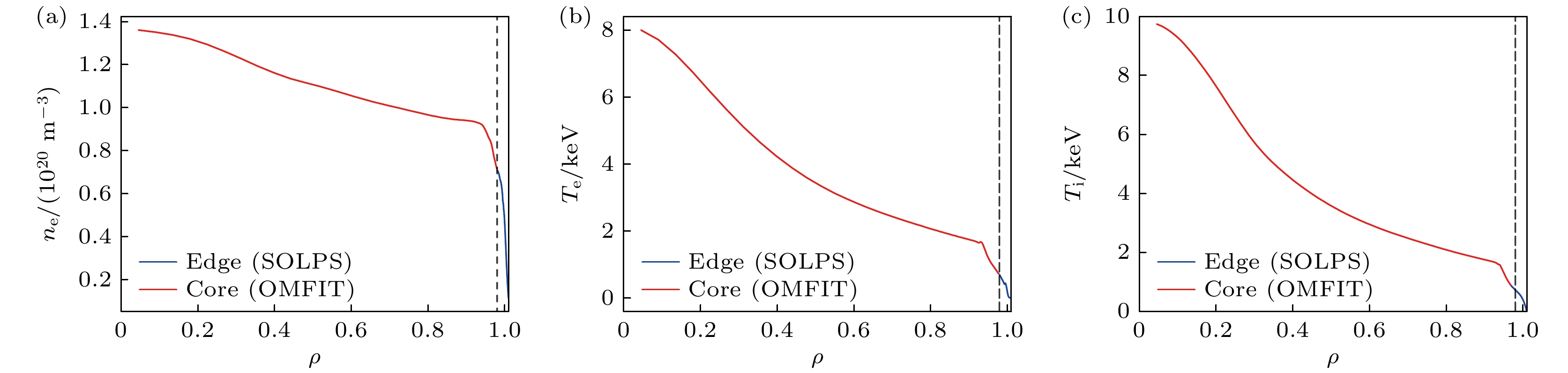
图 2
$ \rho $ = 0—1.01区域参数的径向剖面 (a)电子密度ne; (b)电子温度 Te; 和(c)离子温度Ti; 其中红线代表芯部$ \rho $ = 0—0.98区域参数(OMFIT提供), 蓝线代表边缘$ \rho $ = 0.98—1.01区域参数(SOLPS-ITER模拟), 虚线代表$ \rho $ = 0.98位置Figure 2. Radial profiles in the region
$ \rho $ = 0–1.01: (a) Electron density ne; (b) electron temperature Te; (c) ion temperature Ti. The red line represents the core$ \rho $ = 0–0.98 region parameter (provided by OMFIT), the blue line represents the edge$ \rho $ = 0.98–1.01 region parameters (provided by SOLPS-ITER), and the dashed line represents the$ \rho $ = 0.98 location.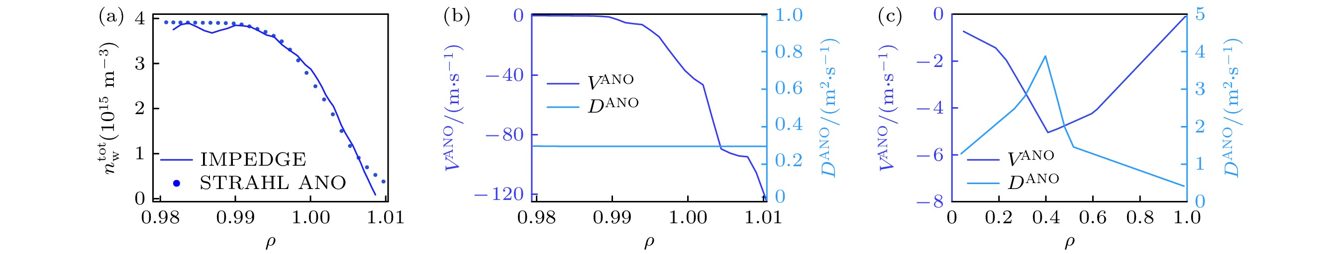
图 3 (a)
$ \rho $ = 0.98—1.01区域的杂质分布, 其中蓝线为IMPEDGE模拟分布, 蓝点为STRAHL模拟分布; (b)$ \rho $ = 0.98—1.01区域湍流扩散系数$ {D}^{{\mathrm{A}}{\mathrm{N}}{\mathrm{O}}} $ 与对流速度$ {v}^{{\mathrm{A}}{\mathrm{N}}{\mathrm{O}}} $ 分布; (c)$ \rho = $ 0—0.98区域湍流扩散系数$ {D}^{{\mathrm{A}}{\mathrm{N}}{\mathrm{O}}} $ 与对流速度$ {v}^{{\mathrm{A}}{\mathrm{N}}{\mathrm{O}}} $ 分布Figure 3. (a) Impurity distribution in the region
$ \rho $ = 0.98–1.01, the blue line represents the IMPEDGE simulation distribution, and the blue dots represent the STRAHL simulation distribution; (b) anomalous diffusion coefficient$ {D}^{{\mathrm{A}}{\mathrm{N}}{\mathrm{O}}} $ and convective velocity$ {v}^{{\mathrm{A}}{\mathrm{N}}{\mathrm{O}}} $ distributions in the region$ \rho $ = 0.98–1.01; (c) anomalous diffusion coefficient$ {D}^{{\mathrm{A}}{\mathrm{N}}{\mathrm{O}}} $ and convective velocity$ {v}^{{\mathrm{A}}{\mathrm{N}}{\mathrm{O}}} $ distributions in the region in the region$ \rho = $ 0–0.98.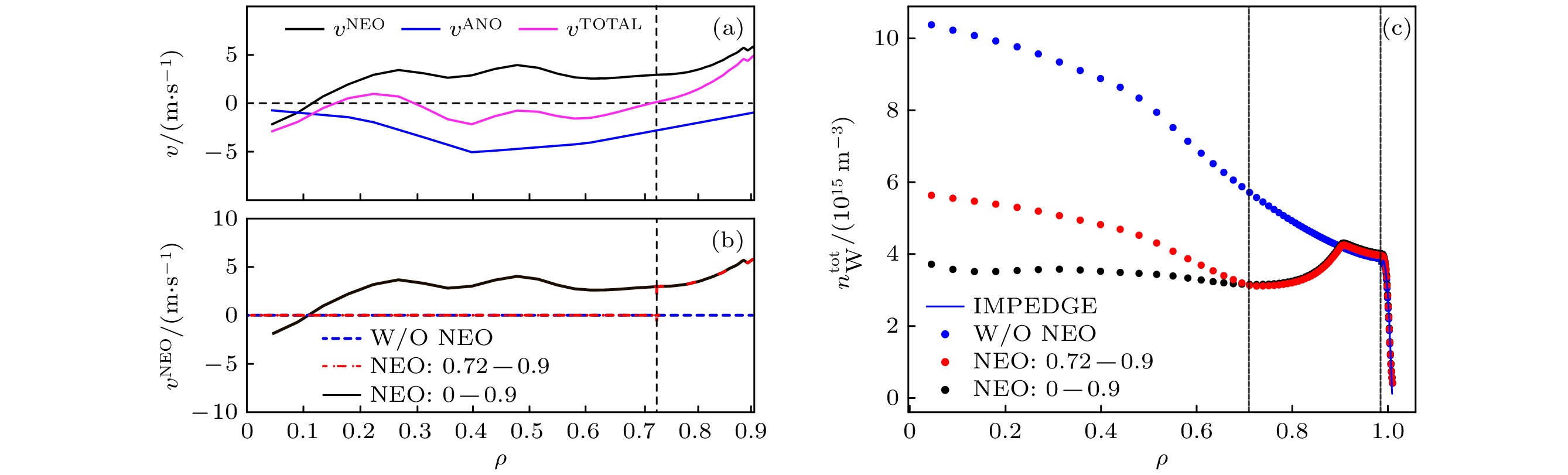
图 4 区域
$ \rho =0—0.9 $ (a)$ {v}^{{\mathrm{N}}{\mathrm{E}}{\mathrm{O}}} $ ,$ {v}^{{\mathrm{A}}{\mathrm{N}}{\mathrm{O}}} $ 和$ {v}^{{\mathrm{T}}{\mathrm{O}}{\mathrm{T}}{\mathrm{A}}{\mathrm{L}}} $ 径向分布; (b) 3种情况下$ {v}^{{\mathrm{N}}{\mathrm{E}}{\mathrm{O}}} $ 分布设置; (c) 区域$ \rho =0—1.01 $ 三种情况下模拟得到的钨杂质密度$ {n}_{{\mathrm{W}}}^{{\mathrm{t}}{\mathrm{o}}{\mathrm{t}}} $ 径向分布, 其中杂质边缘分布均与IMPEDGE一致, 虚线分别表示$ \rho $ = 0.72和$ \rho $ = 0.98所在位置Figure 4. (a) The radial distributions of
$ {v}^{{\mathrm{N}}{\mathrm{E}}{\mathrm{O}}} $ ,$ {v}^{{\mathrm{A}}{\mathrm{N}}{\mathrm{O}}} $ , and$ {v}^{{\mathrm{T}}{\mathrm{O}}{\mathrm{T}}{\mathrm{A}}{\mathrm{L}}} $ ; (b) the setup of$ {v}^{{\mathrm{N}}{\mathrm{E}}{\mathrm{O}}} $ distribution for three different cases in the region$ \rho$ = 0–0.9; (c) radial distribution of tungsten impurity density$ {n}_{{\mathrm{W}}}^{{\mathrm{t}}{\mathrm{o}}{\mathrm{t}}} $ of different cases in the region$ \rho$ = 0–1.01, the$ {n}_{{\mathrm{W}}}^{{\mathrm{t}}{\mathrm{o}}{\mathrm{t}}} $ distributions in the edge region are consistent with those from IMPEDGE. The dashed lines represent the$ \rho =0.72 $ and$ \rho =0.98 $ location.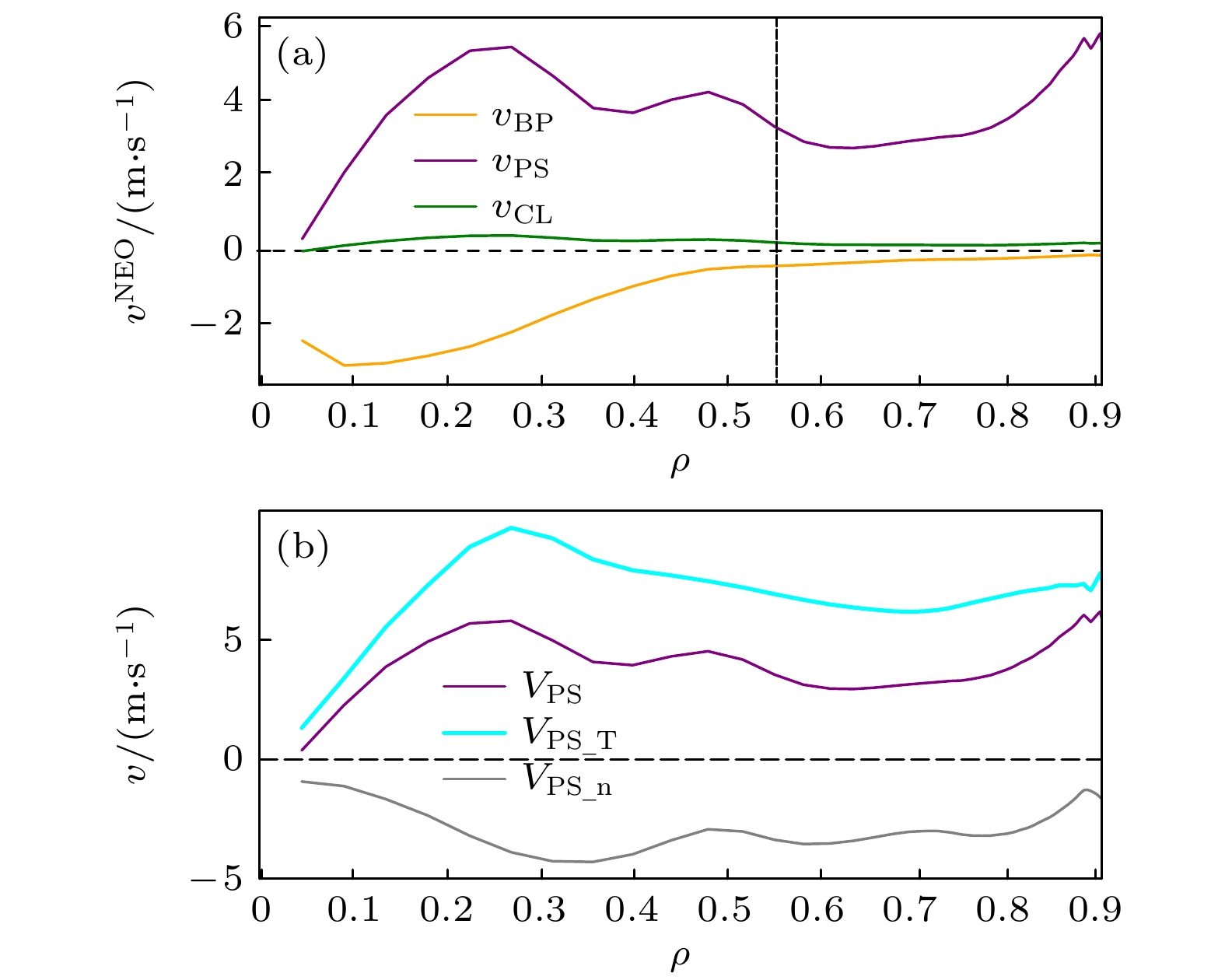
图 5 区域
$ \rho =0—0.9 $ (a)新经典对流速度的3个分量; (b)新经典对流PS分量$ {v}_{{\mathrm{P}}{\mathrm{S}}}^{{\mathrm{N}}{\mathrm{E}}{\mathrm{O}}} $ 及离子温度梯度项$ {v}_{{\mathrm{P}}{\mathrm{S}}\_{\mathrm{T}}}^{{\mathrm{N}}{\mathrm{E}}{\mathrm{O}}} $ 和密度梯度项$ {v}_{{\mathrm{P}}{\mathrm{S}}\_{\mathrm{n}}}^{{\mathrm{N}}{\mathrm{E}}{\mathrm{O}}} $ , 虚线位置为$ \rho =0.55 $ Figure 5. (a) Three components of the neoclassical convective velocity; (b) the neoclassical convective PS component
$ {v}_{{\mathrm{P}}{\mathrm{S}}}^{{\mathrm{N}}{\mathrm{E}}{\mathrm{O}}} $ along with its temperature gradient term$ {v}_{{\mathrm{P}}{\mathrm{S}}\_{\mathrm{T}}}^{{\mathrm{N}}{\mathrm{E}}{\mathrm{O}}} $ and density gradient term$ {v}_{{\mathrm{P}}{\mathrm{S}}\_{\mathrm{n}}}^{{\mathrm{N}}{\mathrm{E}}{\mathrm{O}}} $ in region$ \rho =0$ –0.9, the dashed line represents the$ \rho =0.55 $ location.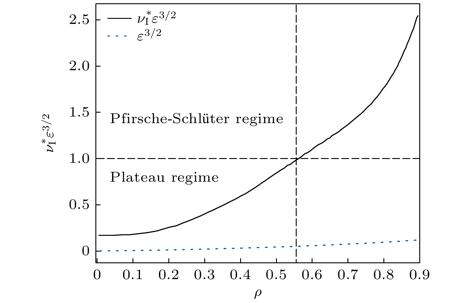
图 6 区域
$ \rho =0—0.9 $ 杂质碰撞率$ {\nu }_{{\mathrm{I}}}^{{\mathrm{*}}} $ 分布, 虚线位置为$ \rho =0.55 $ Figure 6. Impurity collision rate
$ {\nu }_{{\mathrm{I}}}^{{\mathrm{*}}} $ distribution in the region$ \rho$ = 0–0.9 , the dashed line represents the$ \rho =0.55 $ location.表 1 不同
$ {v}^{{\mathrm{N}}{\mathrm{E}}{\mathrm{O}}} $ 使用区域情况下的$ \rho =0 $ 和$ \rho =0.72 $ 处钨密度,$ \rho =0 $ 处钨浓度,$ \rho =0 $ 处钨杂质引起的总辐射损失密度Table 1. In different
$ {v}^{{\mathrm{N}}{\mathrm{E}}{\mathrm{O}}} $ applied region cases, the tungsten density at$ \rho =0 $ and$ \rho =0.72 $ , the tungsten concentration at$ \rho =0 $ and total power radiation loss density by tungsten at$ \rho =0 $ .使用区域 W/O NEO With NEO $ \rho $ = 0.72—0.90With NEO $ \rho $ = 0—0.9$ {n}_{{\mathrm{w}}}^{\rho =0.72} $ (1015 m–3)$ 6.00 $ $ 3.80 $ $ 3.80 $ $ {n}_{{\mathrm{w}}}^{\rho =0} $ (1016 m–3)$ 1.10 $ $ 0.58 $ $ 0.40 $ $ {C}_{{\mathrm{w}}}^{\rho =0} $ (10–5)7.70 4.20 2.50 $ {P}_{{\mathrm{r}}{\mathrm{a}}{\mathrm{d}}}^{\rho =0} $ (MW·m–3)0.26 0.15 0.11  下载: 导出CSV
-
[1] Neu R, Dux R, Geier A, Kallenbach A, Pugno R, Rohde V, Bolshukhin D, Fuchs J C, Gehre O, Gruber O, Hobirk J, Kaufmann M, Krieger K, Laux M, Maggi C, Murmann H, Neuhauser J, Ryter F, Sips A C C, Stäbler A, Stober J, Suttrop W, Zohm H 2002 Plasma Phys. Control. Fusion 44 811 doi: 10.1088/0741-3335/44/6/313 [2] Sang C F, Zhou Q R, Xu G S, Wang L, Wang Y L, Zhao X L, Zhang C, Ding R, Jia G Z, Yao D M, Liu X J, Si H, Wang D Z, the EAST Team 2021 Nucl. Fusion 61 066004 doi: 10.1088/1741-4326/abecc9 [3] Liu B, Dai S Y, Yang X D, Chan V S, Ding R, Zhang H M, Feng Y, Wang D Z 2022 Nucl. Fusion 62 126040 doi: 10.1088/1741-4326/ac95aa [4] Pitts R A, Bonnin X, Escourbiac F, Frerichs H, Gunn J P, Hirai T, Kukushkin A S, Kaveeva E, Miller M A, Moulton D, Rozhansky V, Senichenkov I, Sytova E, Schmitz O, Stangeby P C, De Temmerman G, Veselova I, Wiesen S 2019 Nucl. Mater. Energy 20 100696 doi: 10.1016/j.nme.2019.100696 [5] Gruber O, Sips A C C, Dux R, Eich T, Fuchs J C, Herrmann A, Kallenbach A, Maggi C F, Neu R, Pütterich T, Schweinzer J, Stober J 2009 Nucl. Fusion 49 115014 doi: 10.1088/0029-5515/49/11/115014 [6] Sun Z C, Lian Z W, Qiao W N, Yu J G, Han W J, Fu Q W, Zhu K G 2017 Chin. Phys. Lett. 34 030205 doi: 10.1088/0256-307x/34/12/125203 [7] 张启凡, 乐文成, 张羽昊, 葛忠昕, 邝志强, 萧声扬, 王璐 2024 物理学报 73 185201 doi: 10.7498/aps.73.20240730 Zhang Q F, Le W C, Zhang Y H, Ge Z X, Kuang Z Q, Xiao S Y, Wang L 2024 Acta Phys. Sin. 73 185201 doi: 10.7498/aps.73.20240730 [8] Angioni C 2021 Plasma Phys. Control. Fusion 63 073001 doi: 10.1088/1361-6587/abfc9a [9] Guirlet R, Giroud C, Parisot T, Puiatti M E, Bourdelle C, Carraro L, Dubuit N, Garbet X, Thomas P R 2006 Plasma Phys. Control. Fusion 48 B63 doi: 10.1088/0741-3335/48/12B/S06 [10] Donnel P 2018 Ph. D. Dissertation (Aix-Marseille: Aix Marseille Université [11] Shi S Y, Chen J L, Bourdelle C, Jian X, Odstrčil T, Garofalo A M, Cheng Y X, Chao Y, Zhang L, Duan Y M, Wu M Q, Ding F, Li Y Y, Huang J, Qian J P, Gao X, Wan Y X 2022 Nucl. Fusion 62 066031 doi: 10.1088/1741-4326/ac3e3c [12] Shi S, Chen J, Jian X, Odstrčil T, Clarrisse B, Wu M, Wu M, Duan Y, Chao Y, Zhang L, Cheng Y, Qian J, Garofalo A M, Gong X, Gao X, Wan Y 2022 Nucl. Fusion 62 066040 doi: 10.1088/1741-4326/ac548b [13] Pütterich T, Dux R, Neu R, Bernert M, Beurskens M N A, Bobkov V, Brezinsek S, Challis C, Coenen J W, Coffey I, Czarnecka A, Giroud C, Jacquet P, Joffrin E, Kallenbach A, Lehnen M, Lerche E, de la Luna E, Marsen S, Matthews G, Mayoral M L, McDermott R M, Meigs A, Mlynar J, Sertoli M, van Rooij G 2013 Plasma Phys. Control. Fusion 55 124036 doi: 10.1088/0741-3335/55/12/124036 [14] Lee H, Lee H, Han Y S, Song J, Belli E A, Choe W, Kang J, Lee J, Candy J, Lee J 2022 Phys. Plasmas 29 022504 doi: 10.1063/5.0071192 [15] 赵伟宽, 张凌, 程云鑫, 周呈熙, 张文敏, 段艳敏, 胡爱兰, 王守信, 张丰玲, 李政伟, 曹一鸣, 刘海庆 2024 物理学报 73 035201 doi: 10.7498/aps.73.20231448 Zhao W K, Zhang L, Cheng Y X, Zhou C X, Zhang W M, Duan Y M, Hu A L, Wang S X, Zhang F L, Li Z W, Cao Y M, Liu H Q 2024 Acta Phys. Sin. 73 035201 doi: 10.7498/aps.73.20231448 [16] Mochinaga S, Kasuya N, Fukuyama A, Yagi M 2024 Nucl. Fusion 64 066002 doi: 10.1088/1741-4326/ad3470 [17] Lim K, Garbet X, Sarazin Y, Gravier E, Lesur M, Lo-Cascio G, Rouyer T 2023 Phys. Plasmas 30 082501 doi: 10.1063/5.0157428 [18] Zheng G Y, Cai L Z, Duan X R, Xu X Q, Ryutov D D, Cai L J, Liu X, Li J X, Pan Y D 2016 Nucl. Fusion 56 126013 doi: 10.1088/0029-5515/56/12/126013 [19] Cao C Z, Huang X M, Hu Y, Xie Y F, Zhou J, Qiao T, Gao J M, Cai L Z, Cao Z, HL-2A and HL-3 team 2025 Nucl. Mater. Energy 42 101852 doi: 10.1016/j.nme.2024.101852 [20] Han J Y, He Y X, Zhao D Y, Cai L Z, Wang Y Q, Qian W, Huang W Y, Lu Y, Cai L J, Zhong W L 2025 Nucl. Mater. Energy 42 101861 doi: 10.1016/j.nme.2025.101861 [21] Zhang X L, He Z Y H, Cheng Z F, Yan W, Dong Y B, Liu Y, Deng W, Fu B Z, Shi Z B, Zhang Y P, Shi Y J 2024 Fusion Eng. Des. 208 114674 doi: 10.1016/j.fusengdes.2024.114674 [22] Zhou Q R, Zhang Y J, Sang C F, Li J X, Zheng G Y, Wang Y L, Wu Y H, Wang D Z 2024 Plasma Sci. Technol. 26 104003 doi: 10.1088/2058-6272/ad6817 [23] Zhang Y J, Sang C F, Li J X, Zheng G Y, Senichenkov I Y, Rozhansky V A, Zhang C, Wang Y L, Zhao X L, Wang D Z 2022 Nucl. Fusion 62 106006 doi: 10.1088/1741-4326/ac8564 [24] Dux R 2006 STRAHL User Manual Report [25] Wu Y H, Zhou Q R, Sang C F, Zhang Y J, Wang Y L, Wang D Z 2022 Nucl. Mater. Energy 33 101297 doi: 10.1016/j.nme.2022.101297 [26] Zhou Y, Zheng G Y, Du H L, Li J X, Xue L 2022 Fusion Eng. Des. 182 113222 doi: 10.1016/j.fusengdes.2022.113222 [27] Jirakova K, Kovanda O, Adamek J, Komm M, Seidl J 2019 J. Instrum. 14 C11020 doi: 10.1088/1748-0221/14/11/C11020 [28] Wang J F, Wu B, Wang J, Hu C D 2013 J. Fusion Energy 33 20 doi: 10.1007/s10894-013-9633-x [29] Candy J, Holland C, Waltz R E, Fahey M R, Belli E 2009 Phys. Plasmas 16 060704 doi: 10.1063/1.3167820 [30] Logan N C, Grierson B A, Haskey S R, Smith S P, Meneghini O, Eldon D 2018 Fusion Sci. Technol. 74 125 doi: 10.1080/15361055.2017.1386943 [31] Dux R, Loarte A, Angioni C, Coster D, Fable E, Kallenbach A 2017 Nucl. Mater. Energy 12 28 doi: 10.1016/j.nme.2016.10.013 [32] Dubuit N, Garbet X, Parisot T, Guirlet R, Bourdelle C 2007 Phys. Plasmas 14 042301 doi: 10.1063/1.2710461 [33] Dux R 2004 Ph. D. Dissertation (Garching: Max Planck Institut für Plasmaphysik [34] Wang Y L, Sang C F, Zhao X L, Wu Y H, Zhou Q R, Zhang Y J, Wang D Z 2023 Nucl. Fusion 63 096024 doi: 10.1088/1741-4326/aceb09 [35] 杜海龙, 桑超峰, 王亮, 孙继忠, 刘少承, 汪惠乾, 张凌, 郭后扬, 王德真 2013 物理学报 62 245206 doi: 10.7498/aps.62.245206 Du H L, Sang C F, Wang L, Sun J Z, Liu S C, Wang H Q, Zhang L, Guo H Y, Wang D Z 2013 Acta Phys. Sin. 62 245206 doi: 10.7498/aps.62.245206 [36] Wang Y L, Sang C F, Zhang C, Zhao X L, Zhang Y J, Jia G Z, Senichenkov I Y, Wang L, Zhou Q R, Wang D Z 2021 Plasma Phys. Control. Fusion 63 085002 doi: 10.1088/1361-6587/ac0351 [37] Sang C F, Ding R, Bonnin X, Wang L, Wang D Z, EAST Team 2018 Phys. Plasmas 25 072511 doi: 10.1063/1.5038848 [38] Zhao X L, Sang C F, Zhou Q R, Zhang C, Zhang Y J, Ding R, Ding F, Wang D Z 2020 Plasma Phys. Control. Fusion 62 055015 doi: 10.1088/1361-6587/ab831b [39] Zhou Q R, Sang C F, Xu G L, Ding R, Zhao X L, Wang Y L, Wang D Z 2020 Nucl. Mater. Energy 25 100849 doi: 10.1016/j.nme.2020.100849 [40] Shi S Y, Chen J L, Bourdelle C, Jian X, Odstrčil T, Garofalo A M, Cheng Y X, Chao Y, Zhang L, Duan Y M, Wu M F, Ding F, Qian J P, Gao X 2022 Nucl. Fusion 62 066032 doi: 10.1088/1741-4326/ac3e3b [41] Shi S Y, Jian X, Chan V S, Gao X, Liu X J, Shi N, Chen J L, Liu L, Wu M Q, Zhu Y R, CFETR Physics Team 2018 Nucl. Fusion 58 126020 doi: 10.1088/1741-4326/aae397 [42] Wesson J 2011 Tokamaks (Oxford: Oxford University Press) pp153–161 -
计量
- 文章访问数: 163
- HTML全文浏览数: 163
- PDF下载数: 5
- 施引文献: 0